Parameters of Discrete Random Variables
(How to Find the Mean, Median, Mode, Variance & Standard Deviation of a Discrete Random Variable)
In this section we learn how to find the , mean, median, mode, variance and standard deviation of a discrete random variable.
We define each of these parameters:
- mode
- mean (expected value)
- variance & standard deviation
- median
It is worth spending a bit of time on this section as all that is taught here applies to all discrete random variable probability distributions, such as the Binomial Distribution as well as the Poisson Distribution.
Mode
Given a discrete random variable \(X\), its mode is the value of \(X\) that is most likely to occur.
Consequently, the mode is equal to the value of \(x\) at which the probability distribution function, \(P\begin{pmatrix}X = x \end{pmatrix}\), reaches a maximum.
Example
A discrete random variable \(X\)can take-on the values: \[x = \left \{ 2, \ 3, \ 4, \ 5, \ 6 \right \}\] and has probability distribution function: \[P\begin{pmatrix} X = x \end{pmatrix} = \frac{x^2}{90}\]
- Construct the probability distribution table for \(X\).
- Find the mode of the discrete random variable.
Mean \(\mu \) (or Expected Value \(E\begin{pmatrix}X\end{pmatrix} \))
The expected value of a discrete random variable \(X\) is the mean value (or average value) we could expect \(X\) to take if we were to repeat the experiment a large number of times. It is calculated with: \[E(X) = \sum x.P \begin{pmatrix} X = x \end{pmatrix} \] The expected value is also known as the mean \(\mu \) of the random variable, in which case we write: \[\mu = \sum x.P \begin{pmatrix} X = x \end{pmatrix}\] Note: it doesn't matter whether we refer to \(E(X)\) or \(\mu \), but it is important to know that they both refer to the same thing.
Example
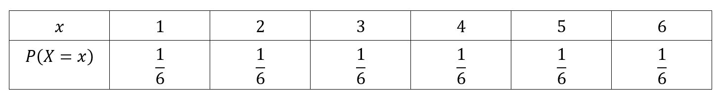
Consider the simple experiment of rolling a single unbiased dice once.
Define the discrete random variable \(X\) as:
\[X:\text{the value obtained when rolling the dice}\]
Find the mean value of this discrete random variable.
Tutorial 1
In the following tutorial we show how to find the mode and the mean of a discrete random variable, using the rules we just read (above).
We do this for a discrete random variable \(X\) that has the following probability distribution table:
Exercise 1
-
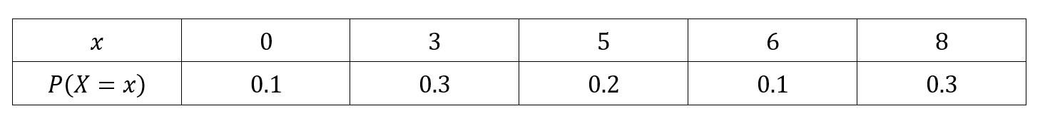
A discrete random variable \(X\) has the following probability distribution table:
- State the mode.
- Calculate this discrete random variable's mean value.
-
A discrete random variable \(X\) can take on the values:
\[x = \left \{ 2, \ 4, \ 6 \right \}\]
and has probability distribution function defined as:
\[P\begin{pmatrix} X = x \end{pmatrix} = \frac{8x - x^2}{40}\]
- Construct a probability distribution table for \(X\).
- State the mode of \(X\).
- Calculate this discrete random variable's mean value.
-
A discrete random variable \(X\) has probability distribution table:
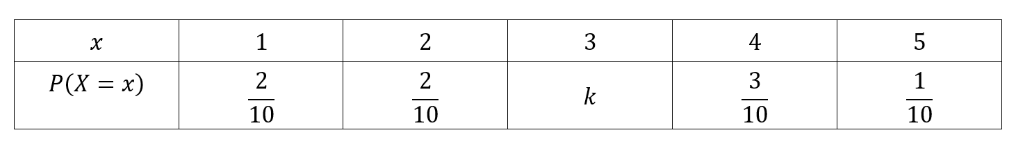
- Find the value of \(k\).
- State the mode of \(X\).
- Calculate the expected value \(E\begin{pmatrix}X\end{pmatrix}\).
Exercise 1 - Answer Key
-
- The Mode is \(X = 2\).
- The mean value is \(\mu = 3.14\) (rounded to 3 significant figures).
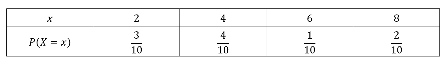
-
-
The probability distribution table is shown here:
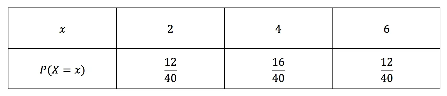
- The mode is \(X = 4\)
- The mean value is \(\mu = 4\)
-
The probability distribution table is shown here:
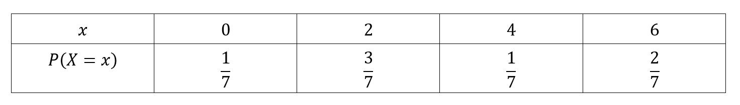
-
- \(k = \frac{2}{10} \quad (=0.2)\)
- The mode is \(X = 4\)
- \(E\begin{pmatrix}X\end{pmatrix} = 2.9\) we could also write \(\mu = 2.9\).
Variance & Standard Deviation
Variance, \(Var\begin{pmatrix}X\end{pmatrix}\) or \(\sigma^2\)
Given a discrete random variable \(X\), we calculate its Variance, written \(Var\begin{pmatrix}X \end{pmatrix}\) or \(\sigma^2\), using one of the following two formula:
Formula 1
\[Var\begin{pmatrix}X \end{pmatrix} = \sum \begin{pmatrix}x - \mu \end{pmatrix}^2 . P\begin{pmatrix} X = x \end{pmatrix}\]
Formula 2
\[Var\begin{pmatrix} X \end{pmatrix} = E\begin{pmatrix}X^2 \end{pmatrix} - \mu^2\] Where: \[E\begin{pmatrix}X^2 \end{pmatrix} = \sum x^2.P\begin{pmatrix} X = x \end{pmatrix}\]Standard Deviation, \(\sigma \)
The standard deviation, \(\sigma\), of a discrete random variable \(X\) tells us how far away from the mean \(\mu \) we can expect the value of \(X\) to be.
We calculate \(\sigma \) using the formula:
\[\sigma = \sqrt{ Var \begin{pmatrix} X \end{pmatrix}}\]
Note: it is important to realize and keep in mind that the value of \(\sigma \) is an average and could be expected to be observed after a sufficiently large number of trials.
Example
A discrete random variable \(X\) can take the values \(x = \left \{ 3, \ 4, \ 6, \ 7 \right \}\) and has a probability distribution function \(P\begin{pmatrix} X = x \end{pmatrix} = \frac{x}{20}\).
- Calculate the mean value of \(X\).
- Calculate the variance and the standard deviation.
Tutorial 2
In tutorial 2 we learn how to calculate the variance and standard deviation of a discrete random variable.
We do this for the following example:
A discrete random variable \(X\) can take the values \(x = \left \{ 1, \ 2, \ 3, \ 4 \right \}\).
It has probability distribution function \(P\begin{pmatrix}X = x \end{pmatrix} = \frac{x}{10}\).
Find: the variance and the standard deviation of \(X\).
Exercise 2
-
A discrete random variable \(X\) has probability distribution function defined as:
\[P\begin{pmatrix} X = x \end{pmatrix} = \frac{x^2}{120}\]
Where \(X\) can take-on the values \(1\), \(3\), \(5\), \(6\) and \(7\).
- Calculate this discrete random variable's mean value.
- Calculate the standard deviation.
-
A discrete random variable \(X\) has the following probability distribution table:
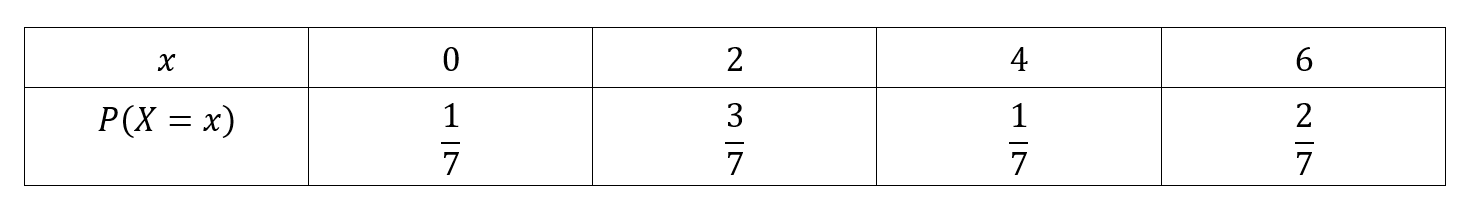
- Calculate the mean value of \(X\).
- Calculate the variance of \(X\).
- Calculate the standard deviation of \(X\)
-
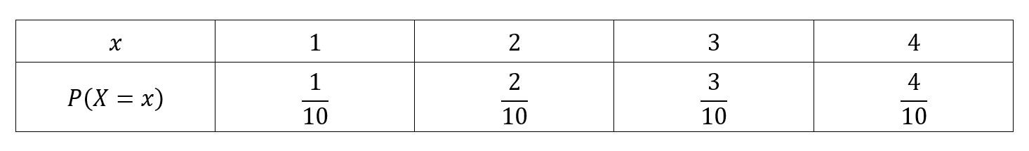
A discrete random variable \(X\) can take-on the values:
\[x = \left \{ 1, \ 2, \ 3, \ 4 \right \}\]
and
has probability distribution function:
\[P\begin{pmatrix} X = x \end{pmatrix} = \frac{x}{10}\]
- Construct a probability distribution table for this discrete random variable.
- State its mode.
- Calculate the mean value of \(X\).
- Calculate the variance of \(X\), hence calculate its standard deviation.
Exercise 2 - Answer Key
-
- The discrete random variable's mean is \(\mu = 5.93\) (rounded to \(2\) dp).
- The standard deviation, rounded to \(2\) decimal places is \(\sigma = 1.22\).
-
- The mean is \(\mu = 3.14\) (rounded to 2 decimal places).
- The variance is \(Var\begin{pmatrix}X\end{pmatrix} = 4.44\) (rounded to 2 decimal places).
- The standard deviation is \(\sigma = 2.11\) (rounded to 2 decimal places).
-
-
The probability distribution table is shown here:
- The mode is \(X = 4\).
- The mean is \(\mu = 3\).
- The variance is \(Var\begin{pmatrix}X \end{pmatrix} = 1\) and standard deviation \(\sigma = 1\).
-
The probability distribution table is shown here:
Median
Given a discrete random variable \(X\) and its cumulative distribution function \(P\begin{pmatrix} X \leq x \end{pmatrix} = F(x)\), the median of the discrete random variable \(X\) is the value \(M\) defined as: \[M = \frac{x_1+x_2}{2}\] Where:
- \(x_1\) is the greatest value \(X\) can take such that: \(P\begin{pmatrix}X \leq x_1 \end{pmatrix} \leq 0.5\).
- \(x_2\) is the smallest value \(X\) can take such that: \(P\begin{pmatrix}X \leq x_2 \end{pmatrix} \geq 0.5\).
The median \(M\) of \(X\) is the middle value.
The probability that \(X\) takes-on a value less than \(M\) is \(0.5\). Similarly, the probability that \(X\) takes-on a value greater than \(M\) is \(0.5\).
In other words there is an equal chance that \(X\) be greater or less than \(M\).
Example
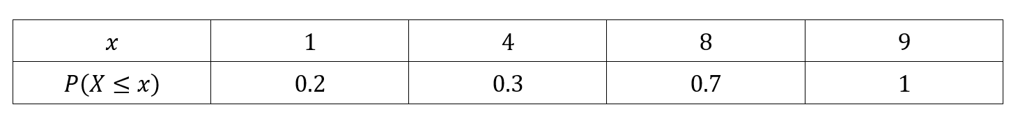
A discrete random variable \(X\) has the following cumulative probability distribution table:
Find the median value of \(X\).
Tutorial 3
In the following tutorial we learn how to find the median of a discrete random variable.
We start by reminding ourselves how to construct a cumulative probability distribution table and then learn how to use it to find the median value.
For this we suppose we're given a discrete random variable \(X\) with the following probability distribution table:
Exercise 3
-
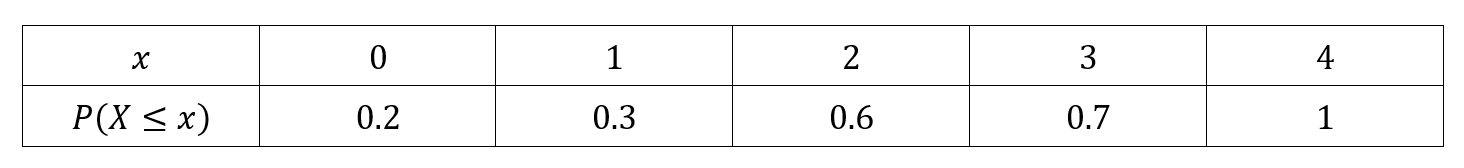
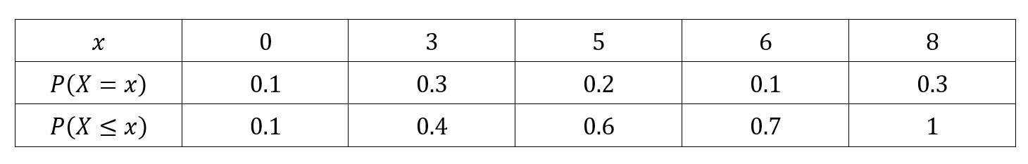
A discrete random variable \(X\) has the following cumulative distribution table:
- Find \(P\begin{pmatrix}X = 4\end{pmatrix}\)
- Find the median value of \(X\).
-
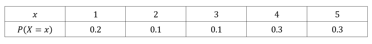
A discrete random variable \(X\) has probability distribution table defined as:
- Construct this random variable's cumulative distribution table.
- Find the median value of \(X\).
-
Given the discrete random variable \(X\), with probability distribution function:
\[P\begin{pmatrix}X = x \end{pmatrix} = \frac{x^2}{90}\]
Where:
\[x = \left \{ 2, \ 3, \ 4, \ 5, \ 6 \right \}\]
- Construct a probability distribution table for \(X\).
- State the mode of \(X\).
- Calculate the mean value of \(X\).
- Calculate this discrete ranom variable's standard deviation.
- Construct a cumulative distribution table for \(X\).
- Find the median value of \(X\).
Exercise 3 - Answer Key
-
- We find \(P\begin{pmatrix}X = 4\end{pmatrix} = 0.1\)
- The median value is \(M = 6\).
-
-
The cululative distribution table is added here, as a third row, to our distribution table:
- The median value is \(M = 4\).
-
The cululative distribution table is added here, as a third row, to our distribution table:
-
-
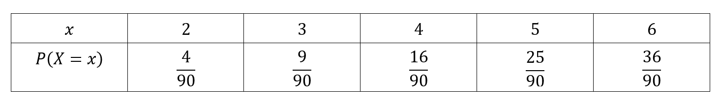
The probability distribution table for \(X\) is shown here:
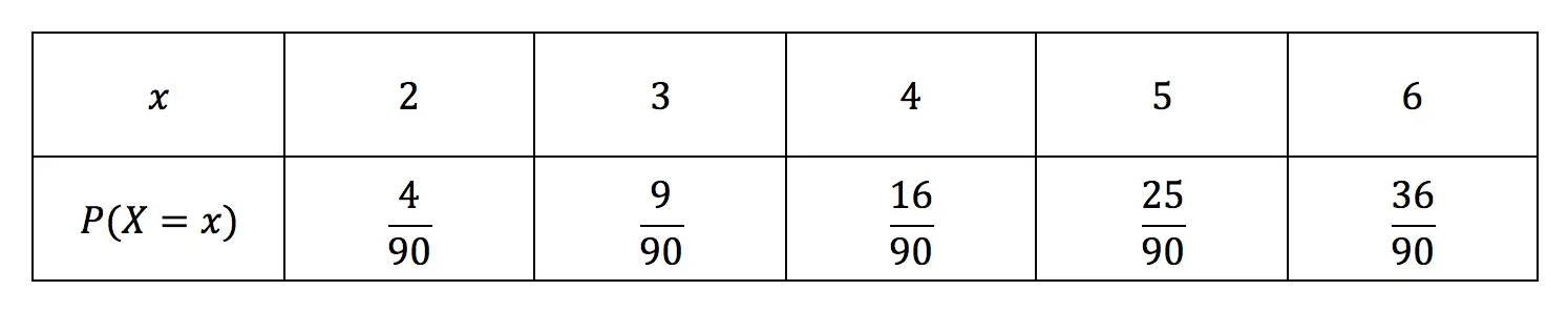
- The mode is \(X=6\)
- The mean value, or expected value, of \(X\) is \(\mu = 4.89\) (rounded to 3 significant figures).
- We find the variance is: \[Var\begin{pmatrix}X \end{pmatrix} = 25.3 - 23.9 = 1.4\] so the standard deviation: \[\sigma = \sqrt{1.4} = 1.18\] (each step was rounded to 3 significant figures)
-
To construct a cumulative distribution table, we've added an \(P\begin{pmatrix}X \leq x \end{pmatrix}\) row to our probability distribution table, as shown here:
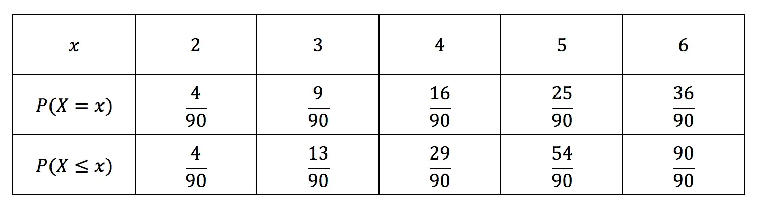
- The median value of \(X\) is \(M = 4.5\).
-
The probability distribution table for \(X\) is shown here:
Scan this QR-Code with your phone/tablet and view this page on your preferred device.

Subscribe Now and view all of our playlists & tutorials.