Parameters of Continuous Random Variable
Continuous random variables, alongside continuous probability distributions have several parameters that we'll need to know how to calculate and interpret.
In this section we learn about:
- the mean
- the median
- the mode
- the variance & standard deviation.
Mean Value \(\mu \) (Expected Value \(E\begin{pmatrix}X\end{pmatrix}\) )
Given a continuous random variable, \(X\), with probability density function (pdf) \(f(x)\), we calculate its mean value \(\mu \) (also known as expected value \(E\begin{pmatrix}X\end{pmatrix}\)) using the formula: \[\mu = \int_{-\infty}^{+\infty}x.f(x)dx\]
Example
A continuous random variable \(X\) has probability density function defined as: \[f(x) = \begin{cases} \frac{x}{4}, \quad 0 \leq x \leq 2 \\ 0, \quad \text{elsewhere} \end{cases}\] Calculate the mean.
Tutorial
The time, in seconds, it takes to re-heat a cup of coffee can be modelled by the continuous random variable \(X\), with probability density function: \[f(x) = \begin{cases} \frac{3}{8}x^2, \quad 0 \leq x \leq 2 \\ 0, \quad \text{elsewhere} \end{cases} \] Calculate the mean amount of time it takes to re-heat a cup of coffee.
Median
The median value of a continuous random variable is the "middle value". That is the value \[\int_{-\infty}^mf(x)dx = \frac{1}{2}\] Graphically, it is the value of \(x\) that splits the area enclosed by the curve \(y=f(x)\) and the \(x\)-axis into two equal areas, both equal to \(0.5\).
Example
The time taken, \(X\) in minutes, for certain bacteria to split into \(2\) distinct bacteria, is believed to follow a continuous probability distribution, with probability density function defined as: \[f(x) = \begin{cases} \frac{3}{8}x^2, \quad 0 \leq x \leq 2 \\ 0, \quad \text{elsewhere} \end{cases}\] Assuming this model is correct, calculate the median time it takes for a bacteria to split in \(2\).
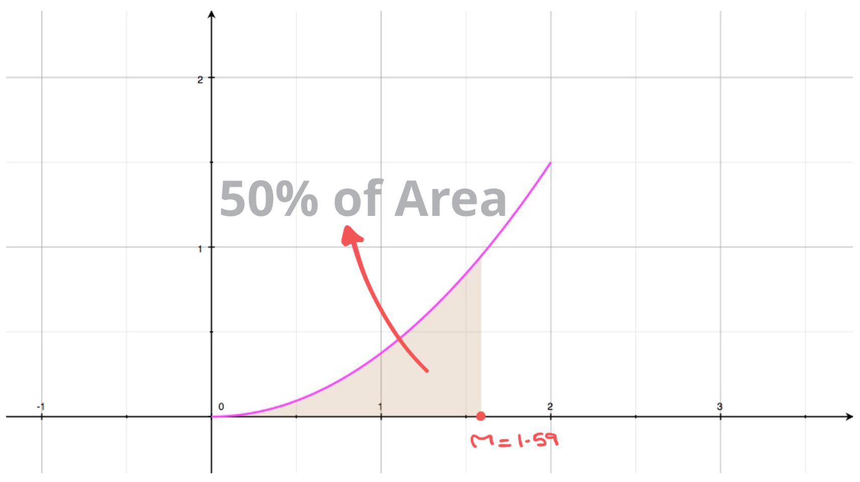 This result is illustrated with the curve shown here.
Mode
The mode of a continuous random variable corresponds to the \(x\) value(s) at which the probability density function reaches a local maximum, or a peak. It is the value most likely to lie within the same interval as the outcome.
Consequently, we'll often find the mode(s) of a continuous random variable by solving the equation: \[f'(x) = 0\] There can be several modes. It is common, when working with continuous random variables, to refer to each local maxima (each peak) as a mode, in which case we say that the continuous random variable is multimodal or plurimodal.
Important
A continuous random variable's mode is not the value of \(X\) most likely to occur, as was the case for discrete random variables.
Remember: for continuous random variables the likelihood of a specific value occurring is \(0\), \(P\begin{pmatrix}X = k \end{pmatrix} = 0\) and the mode is a specific value.
When working with continuous probability distributions the mode is the value most likely to lie within the same interval as the outcome.
Example
The weight (or mass) \(X\), in kg, of newborn babies can, roughly, be approximated by the continuous probability distribution defined as:
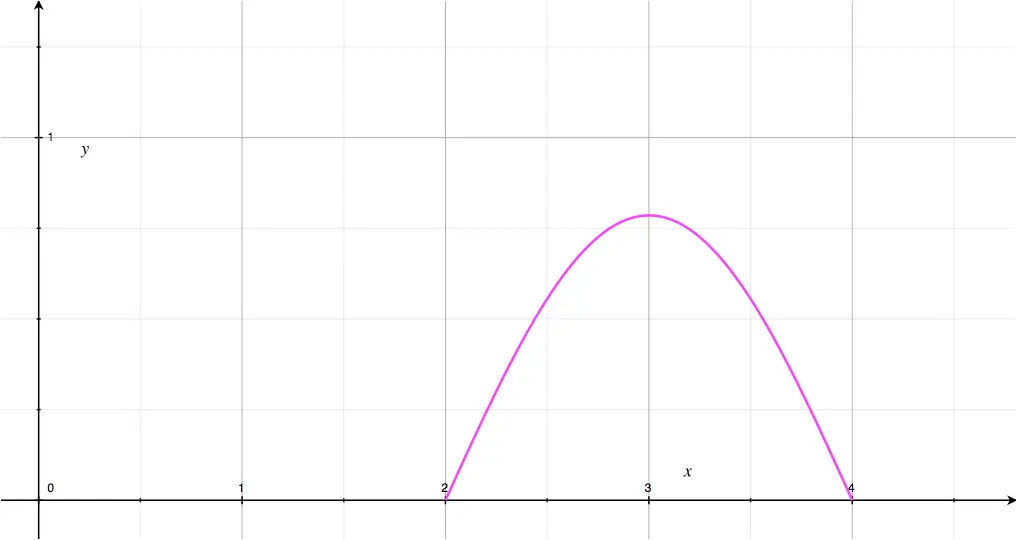 \[f(x) = \begin{cases} \frac{\pi}{4}sin\begin{pmatrix}\frac{\pi (x-2)}{2} \end{pmatrix}, \quad 0\leq x \leq \pi \\
0, \quad \text{elsewhere} \end{cases}
\]
Find the mode (modal value) of the newborn's weight.
\[f(x) = \begin{cases} \frac{\pi}{4}sin\begin{pmatrix}\frac{\pi (x-2)}{2} \end{pmatrix}, \quad 0\leq x \leq \pi \\
0, \quad \text{elsewhere} \end{cases}
\]
Find the mode (modal value) of the newborn's weight.
Note: a more accurate model will be seen when we learn about normal distributions.
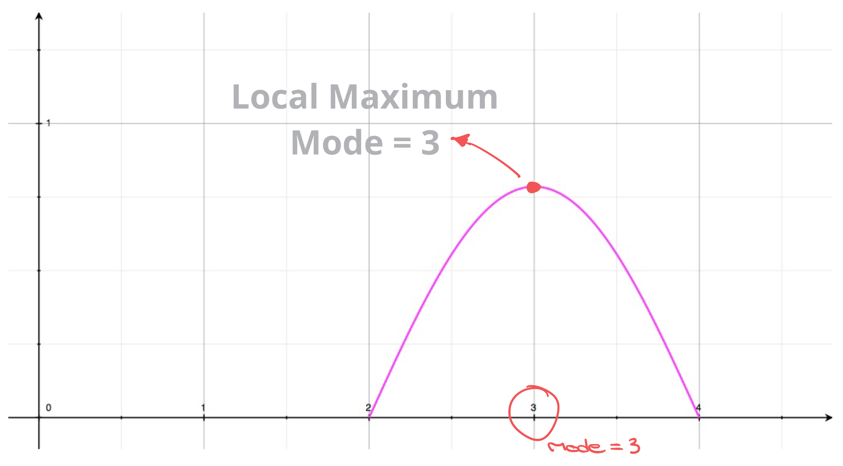 So the solution to the equation \(f'(x)=0\) is:
\[x = 3\]
This is the mode of the continuous random variable:
\[\text{Mode} = 3\]
This result tells us that \(3\) is the value most likely to lie within the range of the outcome of this experiment.
So the solution to the equation \(f'(x)=0\) is:
\[x = 3\]
This is the mode of the continuous random variable:
\[\text{Mode} = 3\]
This result tells us that \(3\) is the value most likely to lie within the range of the outcome of this experiment.Variance & Standard Deviation
Variance, \(Var\begin{pmatrix}X\end{pmatrix}\)
The variance of a continuous random variable is calculated using the formula:
\[Var\begin{pmatrix}X\end{pmatrix} = E\begin{pmatrix}X^2\end{pmatrix} - \mu^2 \]
Where:
\[E\begin{pmatrix}X^2\end{pmatrix} = \int_{-\infty}^{+\infty}x^2.f(x)dx\]
and \(\mu \) is the mean (a.k.a expected value) and was defined further-up.
The variance is the square of the standard deviation, defined next.
Standard Deviation \(\sigma \)
The standard deviation of a continuous random variable is equal to the square root of the variance, that's:
\[\sigma = \sqrt{Var\begin{pmatrix}X\end{pmatrix}}\]
Its value tells us how far, on average, we can expect the value of \(X\) to be from the mean \(\mu\).
Remember \(\sigma \) is an average! If we were to repeat the experiment a large enough number of times then the average distance between the values observed and the mean value would equal to the standard deviation.
Example
The time it takes to open an app, on a smartphone, varies from one device to another.
The time taken \(X\), in seconds, to open/launch the app "Monkey Heaven" has probability density function defined as:
\[f(x) = \begin{cases}
\frac{(x-3)^2}{9}, \quad 0 \leq x \leq 3 \\
0, \quad \text{elsewhere}
\end{cases}\]
- Find the mean value of \(X\)..
- Find the variance.standard deviation.
- Find the standard deviation.
Exercise 1
A continuous random variable \(X\) has probability density function defined as: \[f(x) = \begin{cases} \frac{x^2}{9}, \quad 0\leq x \leq 3 \\ 0, \quad \text{elsewhere} \end{cases}\] Calculate the continuous random variable's:
- mean
- median
- mode
-
- Variance
- Standard Deviation
Answers Without Working
- The mean: \(\mu = 2.25\)
- The median: \(m = \sqrt[3]{\frac{27}{2}} = \frac{3}{\sqrt[3]{2}} \approx 2.38\)
- The mode is \(3\).
-
- The Variance is: \(Var\begin{pmatrix}X \end{pmatrix}=0.3375\)
- The Standard Deviation is: \(\sigma = 0.581\).
Exercise 2
A continuous random variable \(X\) has probability density function defined as: \[f(x) = \begin{cases} \frac{sin(x)}{2}, \quad 0\leq x \leq \pi \\ 0, \quad \text{elsewhere} \end{cases}\] Calculate the continuous random variable's:
- mean
- median
- mode
-
- variance
- standard deviation
Answers Without Working
- The mean: \(\mu = \frac{\pi}{2}\)
- The median: \(m = \frac{\pi}{2}\)
- The mode is \(\frac{\pi}{2}\).
-
- The Variance is: \(Var\begin{pmatrix}X \end{pmatrix}= \frac{\pi^2}{4} - 2 = 0.467\)
- The Standard Deviation is: \(\sigma = 0.684\).
Exercise 3
A continuous random variable \(X\) has probability density function defined as: \[f(x) = \begin{cases} \frac{2}{3}x - \frac{2}{3}, \quad 1\leq x \leq 2 \\ -\frac{x}{3} + \frac{4}{3}, \quad 2\leq x \leq 4 \\ 0, \quad \text{elsewhere} \end{cases}\] Calculate the continuous random variables:
- mean
- median
- mode
-
- variance
- standard deviation
Answers Without Working
-
- The mean: \(\mu = 2.25\)
- The median: \(m = \sqrt[3]{\frac{27}{2}} = \frac{3}{\sqrt[3]{2}} \approx 2.38\)
- The mode is \(3\).
-
- The Variance is: \(Var\begin{pmatrix}X \end{pmatrix}=0.3375\)
- The Standard Deviation is: \(\sigma = 0.581\).