68 95 99.7 Rule for the Normal Distribution
Bell Curves without a Calculator
The 68 95 99.7 rule works for all bell curves. It consists of 3 well-known results/facts that should be known when studying Normal Distributions (a.k.a Guassian Distributions) and Bell Curves.
This rule is commonly used in exams
68 - 95 - 99.7 Rule
Given a continuous random variable \(X\), which follows a normal distribution with mean \(\mu \) and standard deviation \(\sigma \), we know that the total area under the bell curve is equal to 1.
The 68 - 95 - 99.7 rule tells us that:
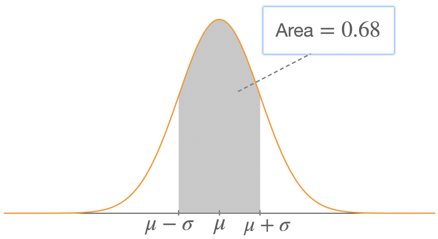
- \(68 \% \) of the total area (which equals to 1) lies within 1 standard deviation of the mean
- \(95 \% \) of the total area lies within 2 standard deviations from the mean
- \(99.7 \% \) of the total area lies within 3 standard deviations from the mean
\(68\% \) : \(1\) Standard Deviation, \(\sigma \)
\(68\% \) of the results fall within 1 standard deviation of the mean \(\mu \); that's between 1 standard deviation to the left of the mean and 1 standard deviation to the right of it.
Example: in the case of \(\mu = 175\)cm and \(\sigma = 7\)cm, we can state that the probability that a man taken at random measures between 168cm and 182cm is 0.68.
\(95\% \) : \(2\) Standard Deviations, \(2 \sigma \)
\(95\% \) of the results fall within 2 standard deviations of the mean \(\mu \).
Example: in the case of \(\mu = 175\)cm and \(\sigma = 7\)cm, we can state that the probability that a man taken at random measures between 161cm and 189cm is 0.95.

\(99.7\% \) : \(3\) Standard Deviations, \(3 \sigma \)
\(99.7\% \) of the results fall within 3 standard deviations of the mean \(\mu \).
Example: in the case of \(\mu = 175\)cm and \(\sigma = 7\)cm, we can state that the probability that a man taken at random measures between 154cm and 196cm is 0.997.
As such we can expect 99.7% of the population to measure between 154cm and 196cm tall.

Example 1
A school's results at the SAT followed a normal distribution with a mean score of \(\mu = 1100\) and standard deviation \(\sigma = 200 \).
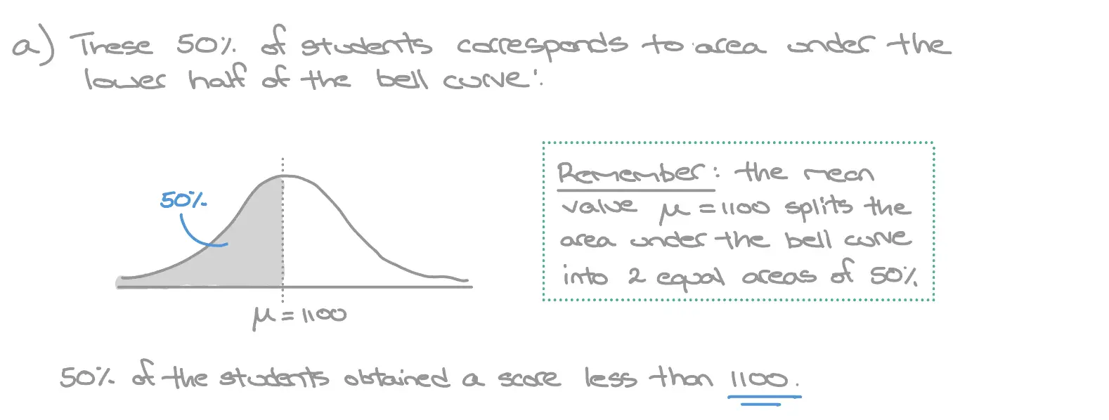
- What score did \(50\%\) of the students get less than?
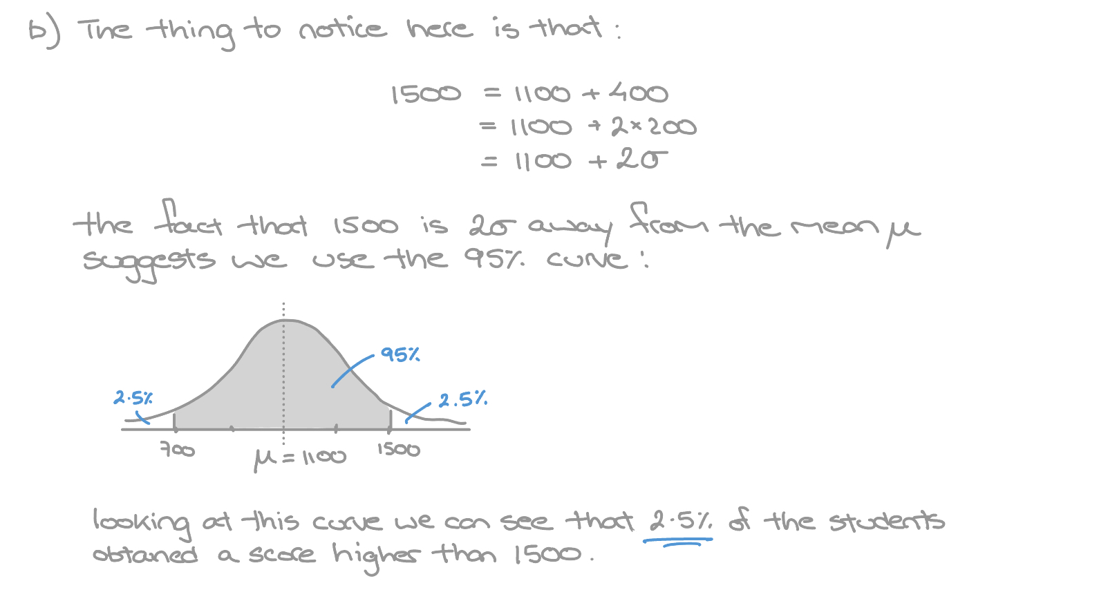
- What percentage of students obtained a score greater than \(1500\)?
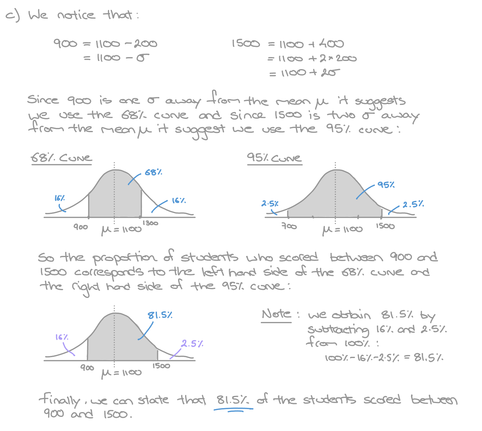
- What percentage of students obtained a score between \(900\) and \(1500\)?
Solution
Example 2
A continuous random variable \(X\) follows a normal distribution with \(\mu = 88\) and \(\sigma = 9\), so \(X \sim N\begin{pmatrix} 88 , 9^2 \end{pmatrix}\).
Without using a calculator, find:
- \(P\begin{pmatrix}X < 97 \end{pmatrix}\)
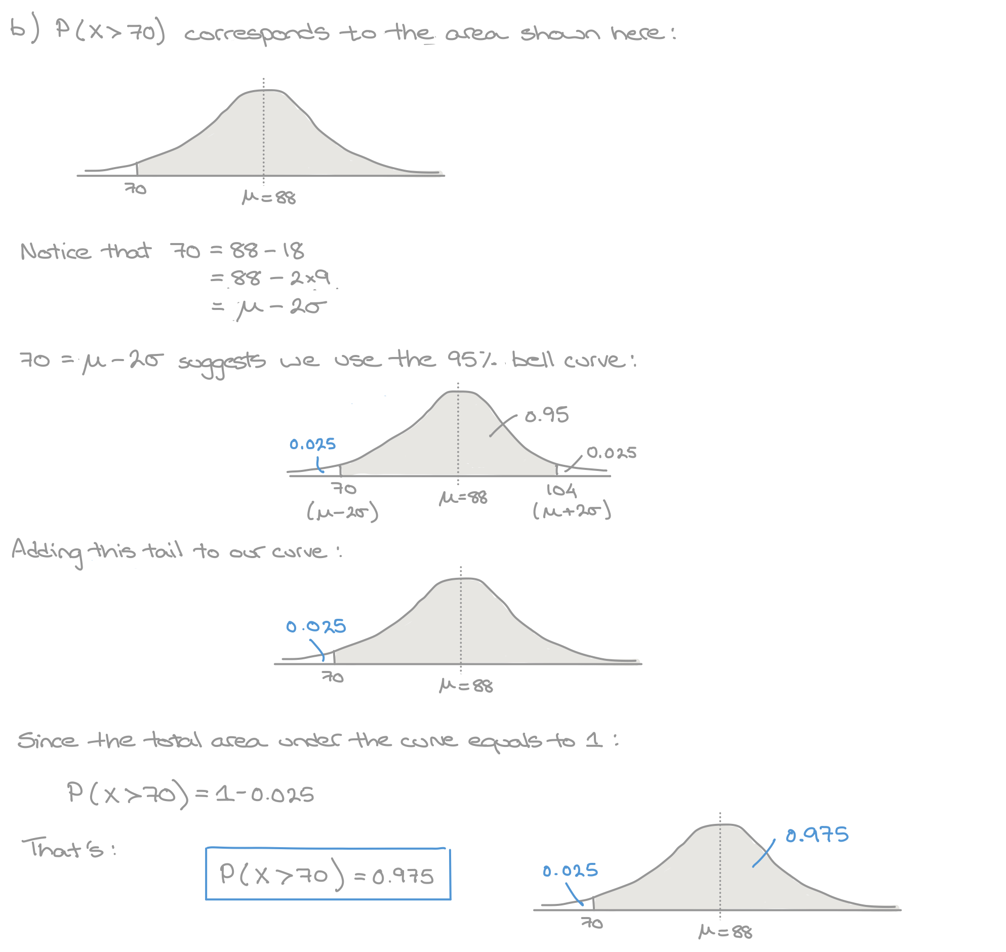
- \(P\begin{pmatrix}X> 70 \end{pmatrix}\)
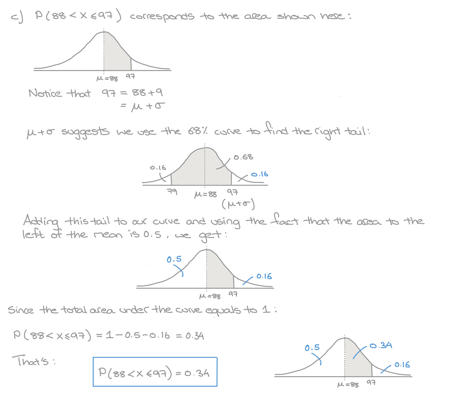
- \(P\begin{pmatrix}88 < X \leq 97 \end{pmatrix}\)
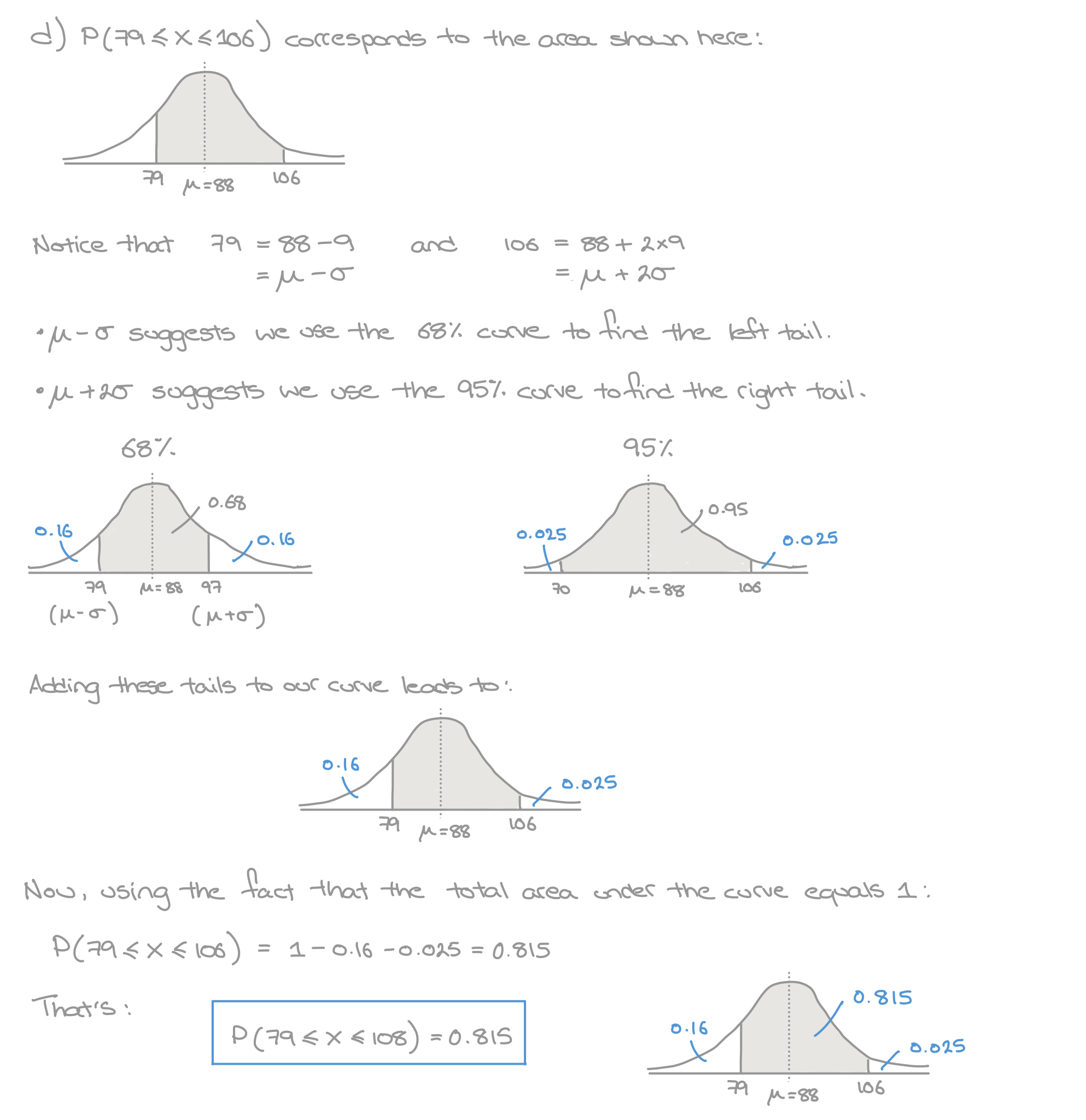
- \(P\begin{pmatrix}79 \leq X \leq 106 \end{pmatrix}\)
Solution

Scan this QR-Code with your phone/tablet and view this page on your preferred device.

Subscribe Now and view all of our playlists & tutorials.