Normal Distribution a.k.a Gaussian Distribution
The Normal Distribution, also known as the Guassian Distribution, is a continuous probability distribution used when working with continuous random variables that are symmetric about their mean value \(\mu\).
Examples of continuous random variables that are normally distributed are: heights of a population, weights of a population, the time taken by members of a population to run 1km, a population's exam scores, ... .
With such examples in mind, continuous random variables that follow a normal distribution are characterised by the fact that the bulk of their most likely values lie close to the mean value and their values become less and less likely the further away one moves from the mean.
Notation
Given a continuous random variable, typically called \(X\), which follows a normal distribution, with mean \(\mu \) and standard deviation \(\sigma\) we'll often say so using the following notation: \[X \sim N \begin{pmatrix} \mu, \sigma^2 \end{pmatrix}\] Where the capital \(N\) refers to the Normal distribution and \(\sigma^2\) refers to the variance, which is equal to the square of the standard deviation \(\sigma^2\).
Example: the height of the adult male population in France follows a normal distrubution with a mean of 175cm and a standard deviation of 7cm. If we define the contniuous random variable \(X\) as the height of the adult male population in France then we could write: \[X\sim N \begin{pmatrix}175, 7^2 \end{pmatrix} \quad \text{or} \quad X\sim N \begin{pmatrix}175, 49 \end{pmatrix}\]
The Bell Curve & the Normal Probability Density Function (normal cdf)
Like all continuous probability distributions, the normal distribution is defined by its probability density function (pdf), we'll often speak of the normal pdf (normal probability density function).
The normal pdf defines the contour, or envelope, of a normal distribution. It is commonly called a bell curve, or guassian curve, whose equation is \(y=f(x)\), where: \[f(x) = \frac{1}{\sigma \sqrt{2\pi}}.e^{-\frac{\begin{pmatrix}x-\mu \end{pmatrix}^2}{2\sigma^2}}, \quad x \in \mathbb{R}\] where :
- \(\sigma \) is the variable's standard deviation
- \(\mu \) is the variable's mean.
Make a Note of It!
To fully define a normal distribution and its bell curve all we need is the two parameters:
- its mean value \(\mu \)
- its standard deviation \(\sigma \)
Bell Curve Characteristics
Bell curves has some key characteristics that we need to know :
- it is symmetrical across the mean \(\mu \)
-
it has 2 points of inflection (2 points at which the concavity changes) when:
- \(x= \mu - \sigma\)
- \(x= \mu + \sigma\)
- the total area enclosed by the bell curve and the x-axis is equal to 1, depending on the context : we could also say it is equal to \(100 \%\)

HOW WE USE BELL CURVES
Say we're considering the adult male population in France which follows a normal distribution with mean height \(\mu = 175 \ \text{cm}\) and standard deviation \(\sigma = 7\ \text{cm}\) and an adult male is randomly selected from the population.
Question: What is the probability that that person measures between 174cm and 180cm ? Or we could also be asked what percentage of the population measures between 174cm and 180cm ? (which would be answered in the same way).
Using the 2 parameters, \(\mu = 175 \ \text{cm}\) and \(\sigma = 7 \ \text{cm}\), we can fully define the normal distribution and its bell curve for the French adult male population.
In fact this bell curve's equation is: \[y = \frac{1}{7\sqrt{2 \pi}}.e^{-\frac{\begin{pmatrix}x-175 \end{pmatrix}^2}{2\times 7^2}}\] (don't worry! there's a function built-in to our calculators to plot this for us).
Once the bell curve is defined, we can find the probability that a randomly selected adult male measures between 174cm and 180cm by calculating the area enclosed by the curve and the x-axis between \(x=174\) and \(x=180\); that's the area shaded in gray on the bell curve.

We'll learn, further down, how to calculate this area with our calculator but for now it's given to us : the area enclosed by this bell curve and the x-axis between \(x=174\) and \(x=180\) is equal to \(0.319\).
This area is equal to the probability we're after. The probability that the randomly selected male measures between 174cm and 180cm is \(0.319\).
Tutorial: Bell Curve, Probabilities, What it's All About
In this tutorial we consider a continuous random variable that follows a normal distribution with mean \(\mu = 88\) and standard deviation \(\sigma = 19\).
TI Nspire CX : NormalCdf functions
In this tutorial we learn how to use the TI Nspire CX Calculator for calculating probabilities.
Now that we have some understanding of what bell curves are and how to use them, we look into the role of the two parameters:
- standard deviation, \(\sigma \)
- mean, \(\mu \)
Role of Standard Deviation \(\sigma \)
The standard deviation, \(\sigma \), is a measure of dispersion: the greater \(\sigma \) the more dispersed the values will be on either side of the mean value \(\mu\).
This can be seen with the 2 bell curves shown here, both have a mean of 100, \(\mu = 100\), but have different standard deviations:
- \(\sigma = 1.5\) leads to the curve being tall and narrow
- \(\sigma = 4\) leads to the curve being wider (and shorter); the values are more dispersed on either side of the mean.

Role of the Mean \(\mu \)
The mean, \(\mu \), tells us the value of \(x\) at which the bell curve is centered on the x-axis; the greater the value of \(\mu \) : the further along the x-axis the bell curve lies.
This can be seen from the 2 bell curves we see here. They both have the same standard deviation, \(\sigma = 2\), so are identical in shape but their mean values are different, \(\mu = 85\) and \(\mu = 100\).

CALCULATING PROBABILITIES
Given a continuous random variable \(X\) that follows a normal distribution, we can use the bell curve to calculate the probability that:
- \(X\) lies between two values, that's: \(P\begin{pmatrix}a \leq X \leq b \end{pmatrix}\); for instance: the probability that a randomly selected man in France measures between 172cm and 183cm.
- \(X\) be less than or equal to a specific value, that's: \(P\begin{pmatrix}X \leq k \end{pmatrix}\); for instance: the probability that a randomly selected man in France measures less than 170cm.
- \(X\) be greater than or equal to a specific value, that's: \(P\begin{pmatrix}X \geq k \end{pmatrix}\); for instance: the probability that a randomly selected man in France measures more than 185cm.
How to Calculate Probabilities using the Bell Curve
- \(P\begin{pmatrix}a \leq X \leq b \end{pmatrix} = \text{Area Enclosed by Curve and x Axis between x = a and x = b}\)
- \(P\begin{pmatrix} X \leq k \end{pmatrix} = \text{Area Enclosed by Curve and x Axis for }x \leq k\)
- \(P\begin{pmatrix} X \geq k \end{pmatrix} = \text{Area Enclosed by Curve and x Axis for }x \geq k\)
Using the example, where the continuous random variable \(X\) is the height of a randomly selected man in France, each of the 3 cases (stated above) is illustrated here:
Case 1: \(P\begin{pmatrix}a \leq X \leq b \end{pmatrix}\)
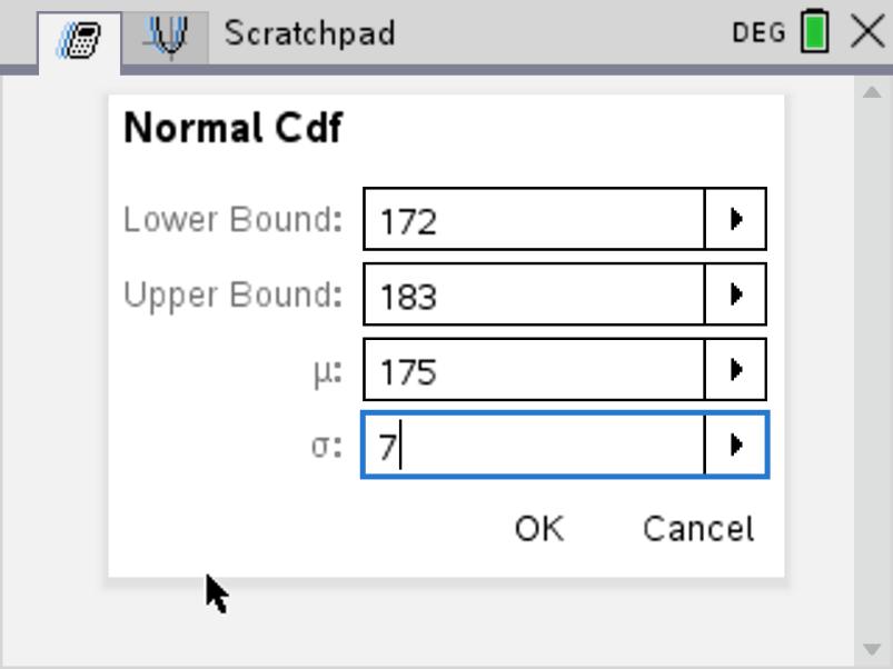
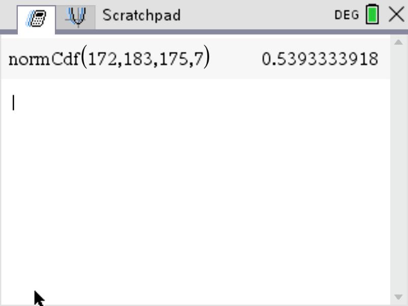
The probability that a randomly selected male, in France, measures between 172cm and 183cm, that's: \[P\begin{pmatrix} 172 \leq X \leq 183\end{pmatrix}\] This probability is equal to the shaded area we see here under the bell curve. That's the area enclosed by the bell curve and the x axis, between the x values 172 and 183.

To calculate this area, and therefore the probability, one way is to use calculus and use the fact that: \[P\begin{pmatrix} 172 \leq X \leq 183\end{pmatrix} = \int_{172}^{183}f(x).dx\] Where, for \(\mu = 175\) and \(\sigma = 7\), \(f(x)\) would be \(f(x) = \frac{1}{7 \sqrt{2\pi}}.e^{-\frac{\begin{pmatrix}x-175 \end{pmatrix}^2}{98}}\). But that would be very difficult.
Instead we use the Normal CDF function on our calculator
- Menu
- Probability
- Distributions
- Normal Cdf
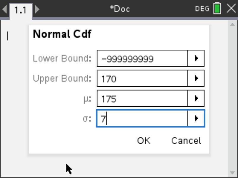
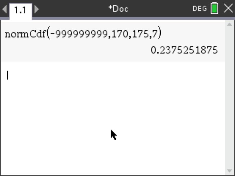
Case 2: \(P\begin{pmatrix} X \leq k \end{pmatrix}\)
The probability that a randomly selected male, in France, measures less than 170cm, that's: \[P\begin{pmatrix} X \leq 170\end{pmatrix}\] This probability is equal to the shaded area we see here under the bell curve. That's the area enclosed by the bell and the x axis for x values less than 170.
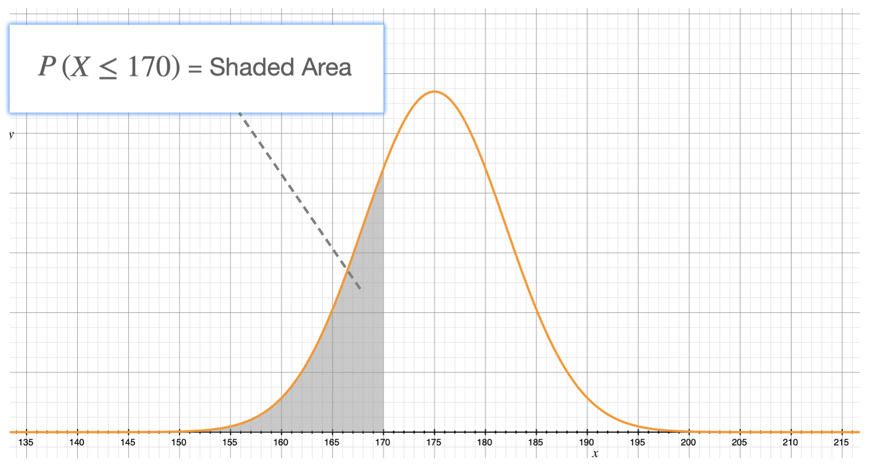
Using calculus, this area and therefore this probability is given by: \[P\begin{pmatrix} X \leq 170 \end{pmatrix} = \int_{-\infty}^{170}f(x).dx\] Using our calculator and the normalCdf function.
In this case:
- the lower bound is \(-\infty\), for which we enter a very large negative number such as -999999999
- the upper bound is
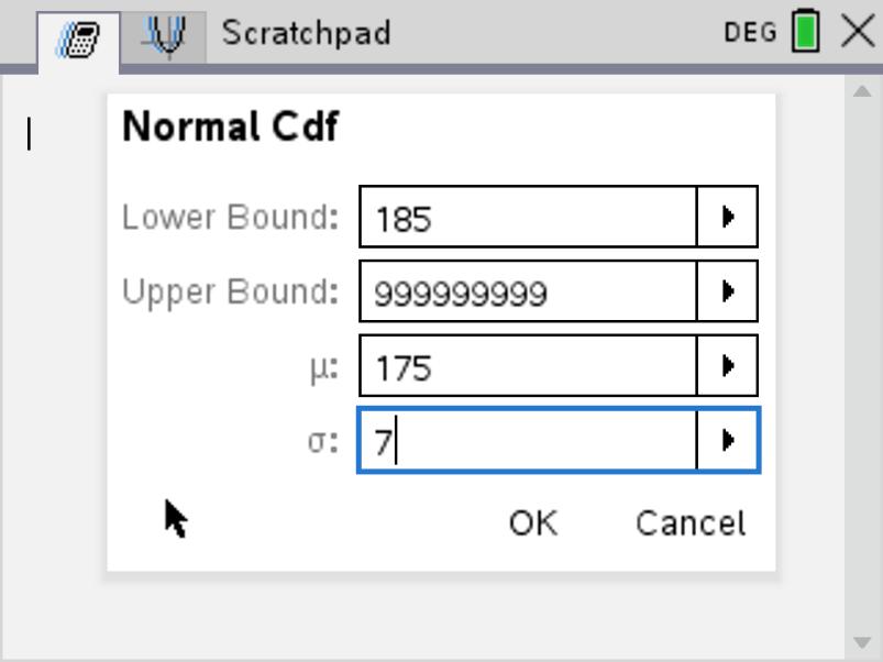
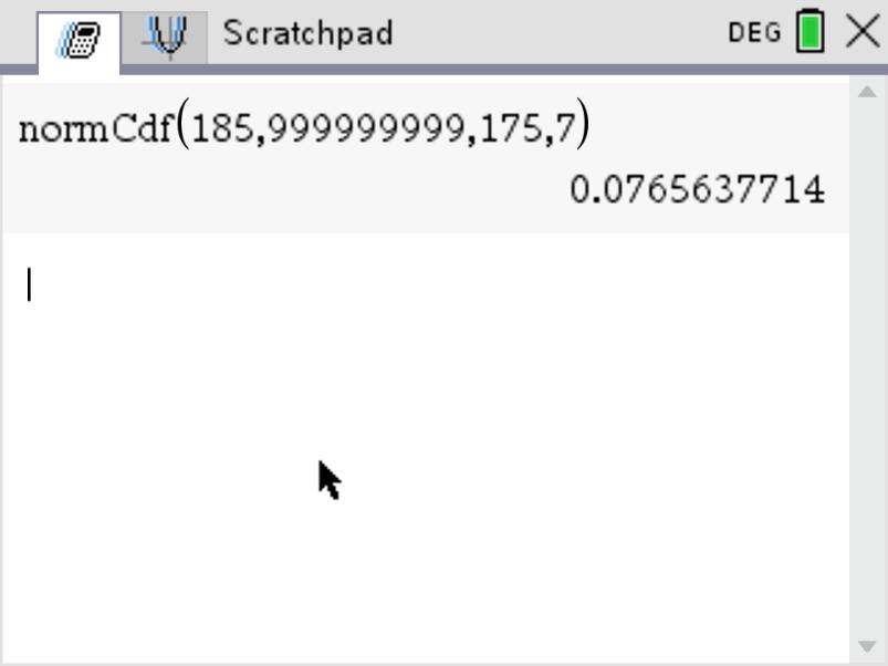
Case 3: \(P\begin{pmatrix} X \geq k \end{pmatrix}\)
The probability that a randomly selected male, in France, measures more than 170cm, that's: \[P\begin{pmatrix} X \geq 185\end{pmatrix}\] This probability is equal to the shaded area we see here under the bell curve. That's the area enclosed by the bell and the x axis for x values greater than 185.
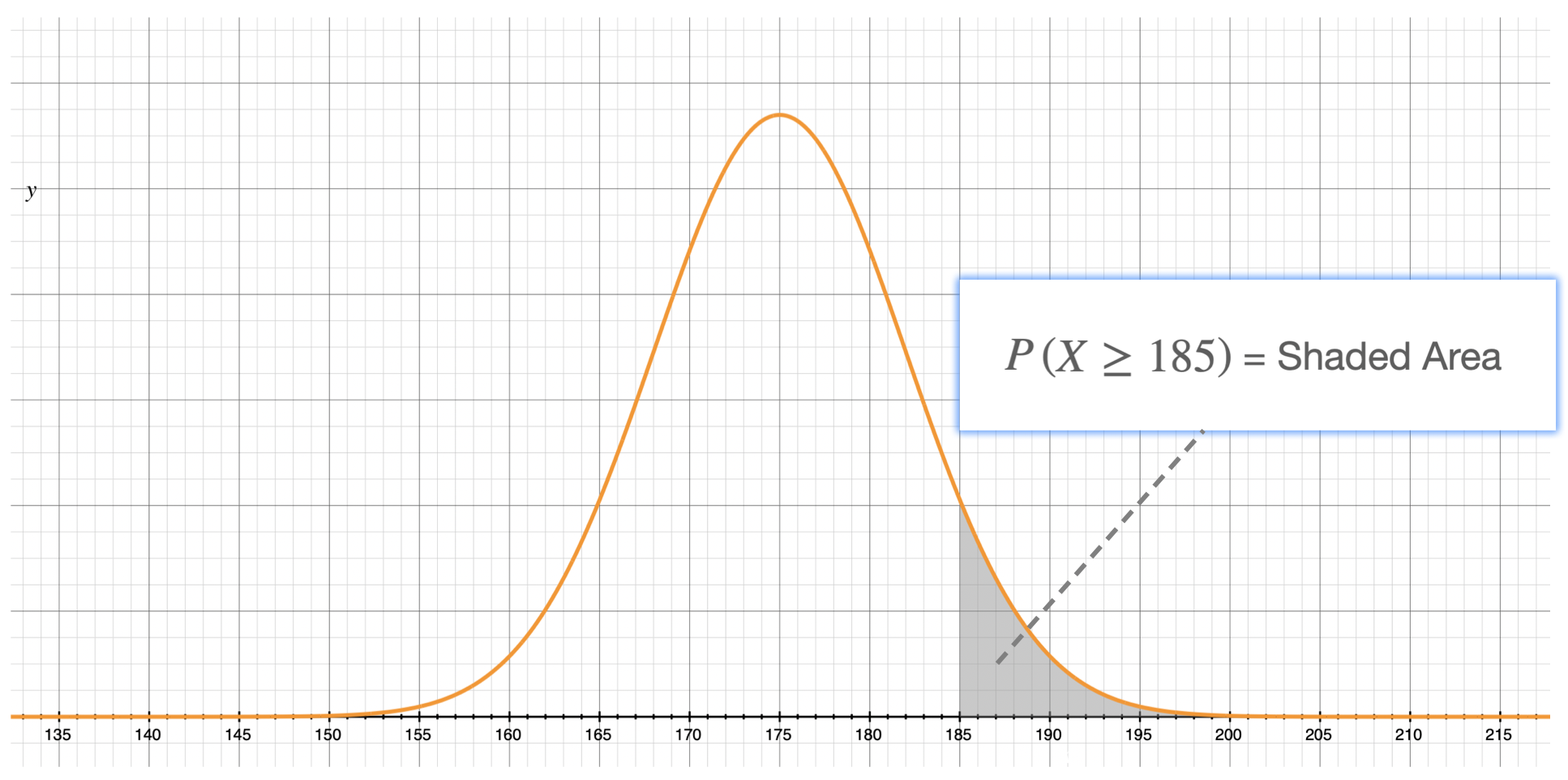
Using calculus, this area and therefore this probability is given by: \[P\begin{pmatrix} X \geq 185 \end{pmatrix} = \int_{185}^{+ \infty}f(x).dx\] Using our calculator and the normalCdf function.
In this case:
- the lower bound is \(185\)
- the upper bound is \(+ \infty\), so we just need to write a very big positive number such as 999999999.
Exam Question
A company produces cartons of milk.
The volume of milk, in ml, that each carton contains can be modeled by a normal distribution with mean 1000 and standard deviation 4.
In the manufacturing process, a carton of milk is rejected (cannot be sold) if it contains a volume less than 995ml.
- Find the probability that a carton selected at random is rejected.
- Estimate the number of cartons that will be rejected from a random sample of 150 cartons.
- Given that a carton is not rejected, find the probability that it contains a volume greater than 1008 ml.
Video Solution
In the following tutorial we see how to solve this exam question in detail.
Scan this QR-Code with your phone/tablet and view this page on your preferred device.

Subscribe Now and view all of our playlists & tutorials.