IB Mathematics: Analysis and Approaches SL — Topic 2 Functions
Graphs of functions
From an equation, a description or a screen to a clear sketch.
Learning goal
Graph functions and communicate their behaviour in clear, labelled sketches.
Syllabus link
IB Mathematics AA SL: SL 2.3. Graphs, sketches and graphing with technology, including sums and differences.
Big idea
A graph shows all the allowed input–output pairs of a function. A screen shows only the part inside its viewing window.
Key relationship
A point on \(y=f(x)\) has coordinates \((x,f(x))\): the input and its output.
This is shared section 2.3 content for AI SL, AA SL and AA HL. The headings 1–9 below organise this lesson; the IB syllabus section is 2.3.
← AA SL Topic 2 Other course editions: AI SL AA HL
What does the equation \(y=f(x)\) tell us?
The notation \(f(x)\), read “f of x”, is the output produced by the input \(x\). Each point \((x,f(x))\) is therefore a pair (input, output). The graph consists of all such pairs for inputs in the domain.
Worked example 1 From a function to points
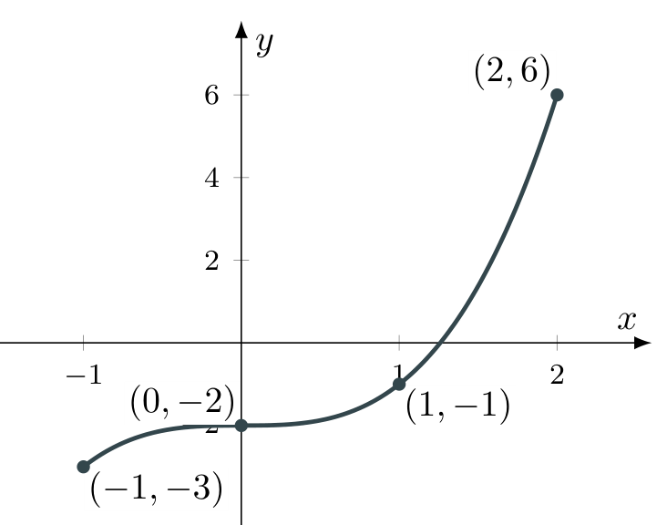
Let \(f(x)=x^3-2\), for \(-1\leq x\leq2\).
- Find the outputs for \(x=-1,0,1,2\).
- Plot the corresponding points and sketch the graph on this domain.
Solution
1. Substitute each input into the function’s equation. For example,
so \((2,6)\) lies on the graph.
| \(x\) (input) | \(-1\) | \(0\) | \(1\) | \(2\) |
|---|---|---|---|---|
| \(f(x)\) (output) | \(-3\) | \(-2\) | \(-1\) | \(6\) |
2. Plot the pairs and use the function’s equation to guide a smooth curve. A table gives sample points; it does not by itself tell us everything between them.
The filled endpoints show that \(x=-1\) and \(x=2\) are included. Do not continue this graph beyond its stated domain.
Drawing and sketching clearly
2.1 Draw or sketch?
| Command | Draw | Sketch |
|---|---|---|
| Purpose | An accurate graph, drawn to scale. | The correct overall shape and relationships. |
| How? | Choose a scale, plot points accurately and join appropriately. Use a ruler for straight lines. | Show the important features in the correct order and relative positions; exact scale is not required. |
| Both need | Labelled axes and relevant features. Include coordinates, units and function names where appropriate. | |
Worked example 2 Sketching from given information
A smooth, continuous graph \(y=h(x)\), defined for all real \(x\), has:
- intercepts \((-2,0)\), \((0,0)\) and \((2,0)\);
- a local maximum at \((-1,2)\) and a local minimum at \((1,-2)\);
- increasing behaviour for \(x<-1\) and \(x>1\), and decreasing behaviour for \(-1<x<1\).
- Sketch one possible graph, labelling all the given points.
- Explain why these facts do not determine a unique function.
Solution
1. Place the intercepts and turning points first. Then draw a smooth curve that rises, falls and rises in the stated intervals.
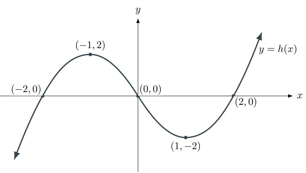
2. Many smooth curves can pass through these points with the stated behaviour. The facts constrain the graph but do not specify every output.
2.2 Show the domain on your sketch
The domain tells us which inputs belong to the function. Your sketch must communicate this, even when the calculator display does not mark the endpoints clearly.
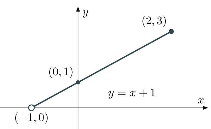
A filled circle includes the point: use it at an endpoint with \(\leq\) or \(\geq\).
An open circle excludes the point: use it at a finite endpoint with \(<\) or \(>\).
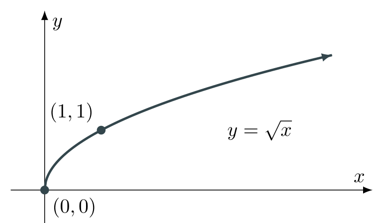
An arrow on the curve shows that the graph continues beyond the part drawn.
A. One excluded and one included endpoint
B. A graph that continues to the right
C. An excluded input inside the view: do not join separate branches
For the supplied graph \(y=\dfrac{1}{x-1}\), the input \(x=1\) is not allowed. The two branches must stay separate.
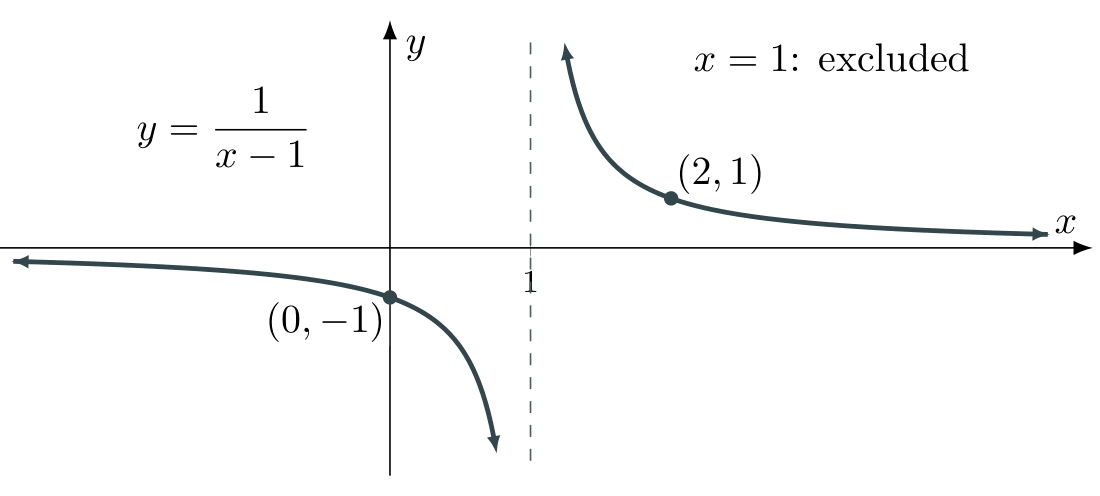
The dashed line is a guide, not part of the graph. Do not draw a vertical curve segment across the gap. An excluded input can also produce a hole in other examples; the graph above has separate branches.
Sketching from a real situation
The context tells us what the axes mean, which inputs are allowed and how the graph should behave. A constant rate gives a straight segment; a constant value gives a horizontal segment.
Worked example 3 Water in a tank
A tank initially contains 120 litres of water. During the first 4 minutes, water is removed at a constant rate until 40 litres remain. The volume stays unchanged for 2 minutes. Water is then added at a constant rate, reaching 100 litres at \(t=10\) minutes.
- State the coordinates at the start and at each change of stage.
- Sketch the volume \(V\) against time \(t\), for \(0\leq t\leq10\).
- Explain the meaning of the horizontal segment.
Solution
1. The input is time and the output is volume. The stage endpoints are
The waiting period ends at \(t=4+2=6\) minutes, not at \(t=2\).
2. Label both quantities and their units. Join the points with straight segments because each stage has a constant rate of change.
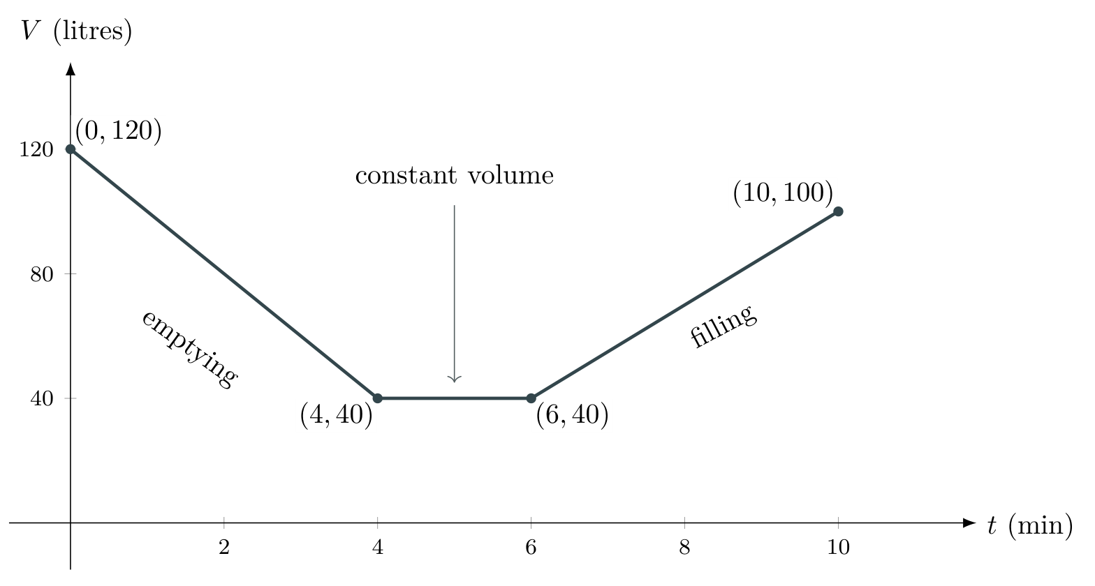
3. Between \(t=4\) and \(t=6\), the volume stays at 40 litres. Time continues to pass even though the volume does not change.
Graphing and checking a function with technology
A graphing calculator (GDC) plots the function you enter. Its window controls which part of the graph is visible; a domain restriction controls which inputs are allowed.
Worked example 4 Set up and check a graph GDC
Consider \(f(x)=x^3-3x+1\), with domain \(-2\leq x\leq2\).
- Enter the function and restrict its domain. [4.1]
- Choose a suitable window and use a table to find the outputs at \(x=-2,-1,0,1,2\). [4.2]
- Sketch the graph on paper, using the supplied features in Section 5. [Section 5]
One example throughout: keep the same function and domain for Tasks 1–3. The references above lead to each solution.
4.1 Enter the function and restrict its domain
Solution — Task 1
Enter the function. Open Scratchpad Graphs and type \(x^3-3x+1\). Press Ctrl, then the = half of the key below it—not trig—to open the symbol palette.
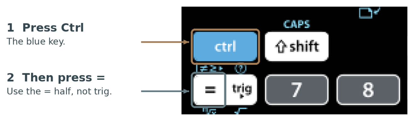
Insert the vertical bar. Select \(\vert\) at the bottom right of the palette. It means “such that” and separates the function’s expression from its domain condition. The highlighted inequalities specify the bounds.
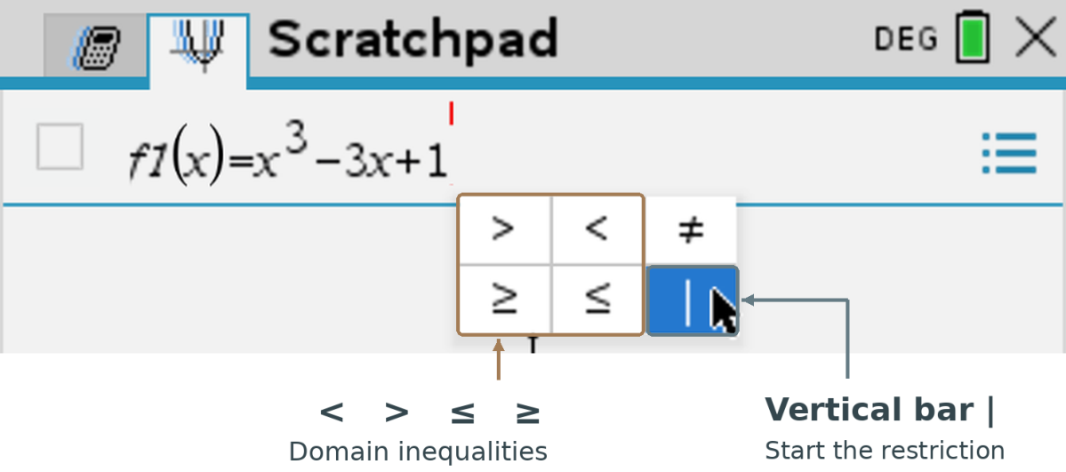
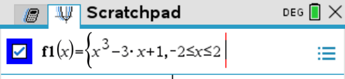
Complete the condition \(-2\leq x\leq2\). After the bar, type \(-2\). Reopen the palette with Ctrl + =, select \(\leq\) (bottom middle), and type \(x\). Reopen the palette again, select \(\leq\), and type \(2\). Check the completed entry, then press Enter:
4.2 Choose the window and check the outputs
Worked example 4 — continued. Keep \(f(x)=x^3-3x+1\) on \([-2,2]\); use the entry from 4.1.
Solution — Task 2
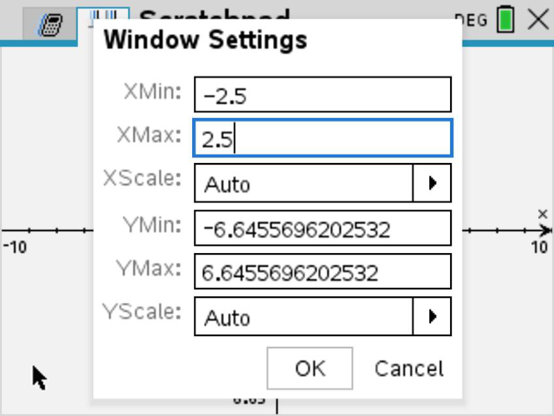
Choose the viewing window. Choose . Set XMin to \(-2.5\) and XMax to \(2.5\), then select OK. In the screenshot, the existing vertical bounds, approximately \(-6.65\) and \(6.65\), already show the whole curve.
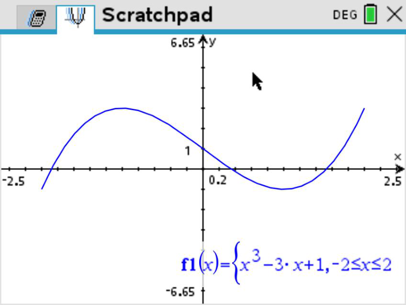
Use a table to check the outputs.
- Press Ctrl + T to show the graph and table together.
- In the table pane, use : set Table Start to \(-2\), Table Step to \(1\), and both columns to Auto.
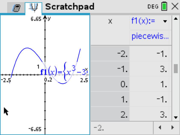
Check the table by substitution. For example,
| \(x\) | \(-2\) | \(-1\) | \(0\) | \(1\) | \(2\) |
|---|---|---|---|---|---|
| \(f(x)\) | \(-1\) | \(3\) | \(1\) | \(-1\) | \(3\) |
The piecewis... label reflects how the calculator stores the restricted function. The table still evaluates the same function on \([-2,2]\).
From the calculator screen to paper
Worked example 4 — continued. Task 3: finish the same cubic example from 4.1–4.2.
Task 3
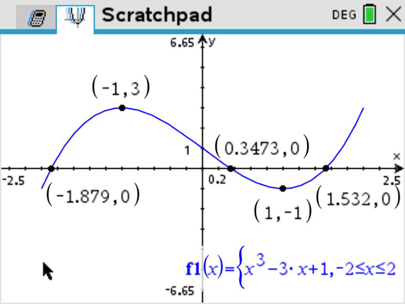
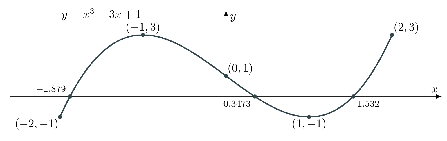
Sketch \(y=x^3-3x+1\) on \([-2,2]\), using the screen and the following supplied features:
- endpoints \((-2,-1)\), \((2,3)\); vertical-axis intercept \((0,1)\);
- local maximum \((-1,3)\) and local minimum \((1,-1)\);
- horizontal-axis crossings at \(x\approx-1.879,\;0.3473,\;1.532\).
These features are supplied here so we can focus on the sketch. Finding them with calculator analysis tools belongs to IB syllabus section 2.4.
Return to the graph pane and press Ctrl + T to remove the table. Compare the initial graph with the screen on which the key features have been identified.
Solution — Task 3
Transfer the graph to paper. Mark the points, preserve the order of the crossings and turns, and use filled endpoints at \(x=-2\) and \(x=2\). The window extends to \(\pm2.5\), but the domain remains \([-2,2]\). A different scale on paper can make the sketch clearer.
Revisit Worked example 4
TI-Nspire CX Essentials for IB Maths — Part 1
Review graphing, window settings, domain restrictions and tables. The tutorial also evaluates \(f(1.5)\).
Adding and subtracting functions
6.1 Combine outputs on the common domain
To form a sum or difference, use the same input in both functions and combine their outputs:
Worked example 5 Check the common domain first
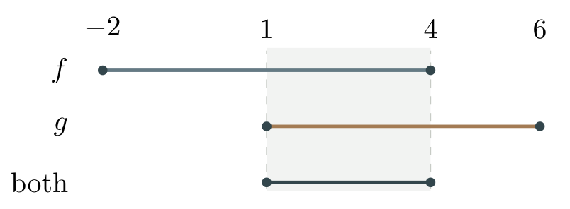
Suppose \(f\) is defined on \([-2,4]\), and \(g\) on \([1,6]\).
- State the domain of \(f+g\) and \(f-g\).
Solution — Task 1
Both outputs exist only for \(1\leq x\leq4\). So both new functions have domain \(\boxed{[1,4]}\).
The common domain is the overlap, not the combined span from \(-2\) to \(6\). Both endpoints are included here.
6.2 Build and check the new functions
Worked example 6 Part A: prepare the functions
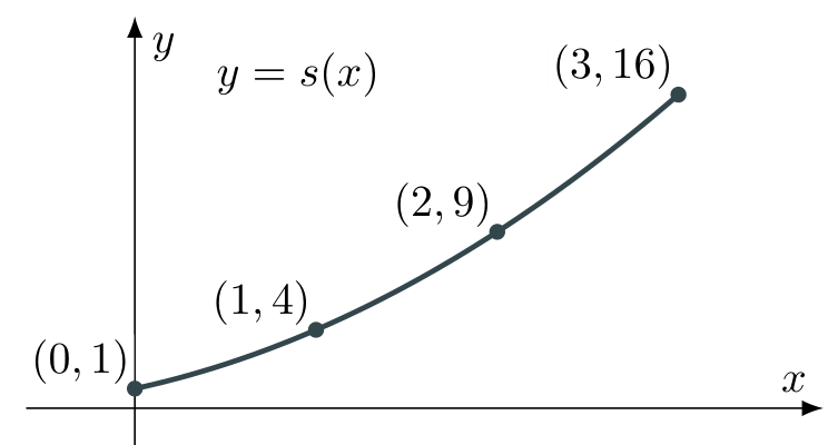
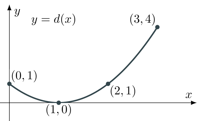
Let \(f(x)=x^2\) and \(g(x)=x+2\), both on \(-2\leq x\leq2\). Define \(s=f+g\) and \(d=f-g\).
- Find \(s(1)\) and \(d(1)\), and interpret the resulting points.
- Find expressions for \(s(x)\) and \(d(x)\).
- Complete a table for \(x=-2,-1,0,1,2\).
Solution
1. First find the two outputs: \(f(1)=1^2=1\) and \(g(1)=1+2=3\). Then
Thus \((1,4)\) lies on \(y=s(x)\), and \((1,-2)\) lies on \(y=d(x)\). In both cases, the input is still \(1\).
2. Substitute the complete expressions, using brackets when subtracting:
3. Add or subtract within each column; never combine different inputs.
| \(x\) | \(-2\) | \(-1\) | \(0\) | \(1\) | \(2\) |
|---|---|---|---|---|---|
| \(f(x)\) | \(4\) | \(1\) | \(0\) | \(1\) | \(4\) |
| \(g(x)\) | \(0\) | \(1\) | \(2\) | \(3\) | \(4\) |
| \(s(x)=f(x)+g(x)\) | \(4\) | \(2\) | \(2\) | \(4\) | \(8\) |
| \(d(x)=f(x)-g(x)\) | \(4\) | \(0\) | \(-2\) | \(-2\) | \(0\) |
Difference is signed: \(f-g\) is positive where \(f>g\), zero where \(f=g\), and negative where \(f<g\). It is not always a positive distance.
Continue with Part B in Section 7. Keep these functions and this table. Part B has five new tasks, numbered 1–5 to match subsections 7.1–7.5.
Sums and differences: from calculator to paper
Worked example 6 Part B: calculator to paper GDC
Continue with \(f(x)=x^2\) and \(g(x)=x+2\), both on \([-2,2]\), from Part A (6.2).
- Plot \(f_1=f\) and \(f_2=g\) on the given domain; choose a suitable window. [7.1]
- Form and graph the sum \(f_3=f_1+f_2\). [7.2]
- Hide the original curves and graph the difference \(f_4=f_1-f_2\). [7.3]
- Evaluate \(f_3(1)\) and \(f_4(1)\); interpret the results as points on the graphs. [7.4]
- Sketch both new graphs on paper, labelling the features supplied in 7.5. [7.5]
Tasks 1–5 match 7.1–7.5. Keep the same functions and domain throughout Part B.
7.1 Plot the original functions
Solution — Task 1
Enter the two original functions. In Scratchpad Graphs, use f1 for \(f\) and f2 for \(g\). Replace the earlier example’s entries if necessary. Enter the following right-hand sides, pressing Enter after each:
The vertical bar means “such that”; insert it using Ctrl + =. To open another function-entry line, choose .

f1.
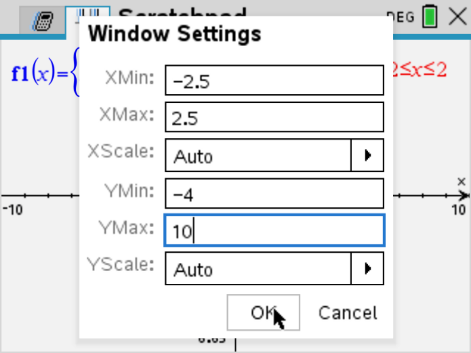
f2.Choose a window for all four graphs. Use and set
Leave both scales on Auto, then select OK.
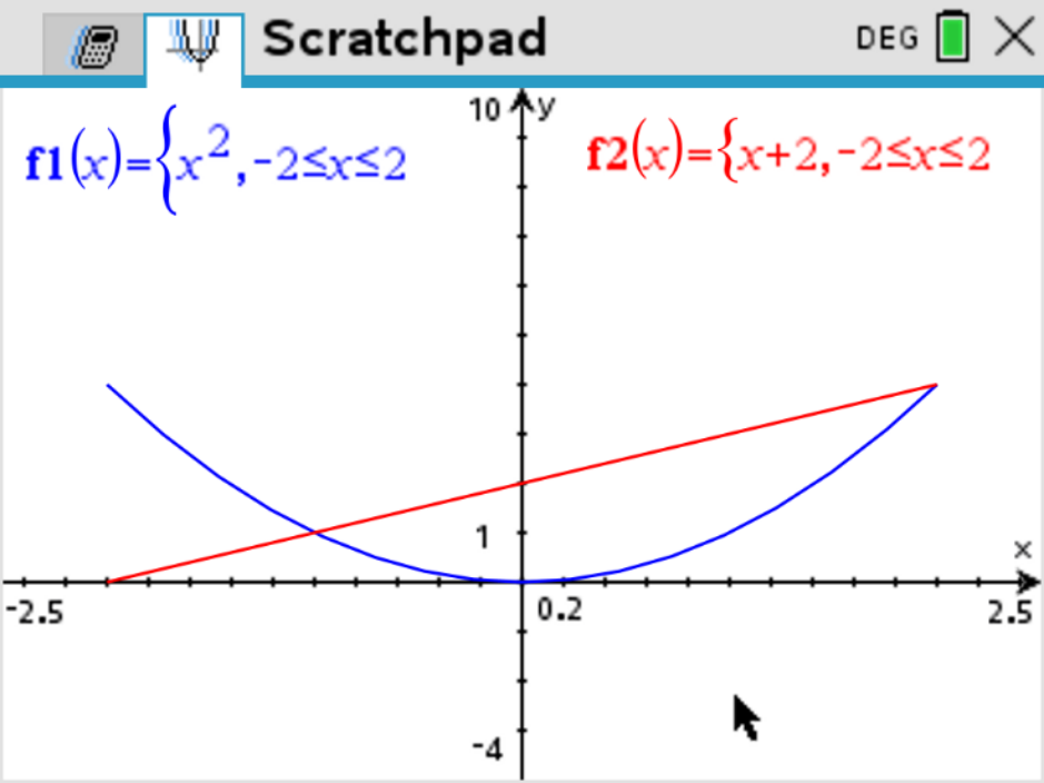
f1; the line is f2.7.2 Recall the functions and form the sum
Worked example 6 — continued. Part B. Keep \(f_1(x)=x^2\) and \(f_2(x)=x+2\), each on \([-2,2]\).
Solution — Task 2
The var key is directly above 9. It opens the list of available stored variables and functions. We will use it both in a graph entry and later on the calculator page.
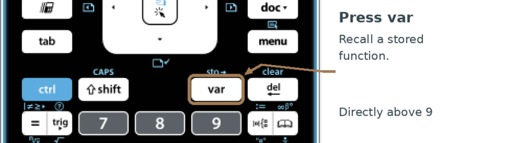
Define the sum as \(f_3(x)=f_1(x)+f_2(x)\).
- Open the next function-entry line,
f3(x)=. - Press var, select
f1, and insert it. Typexinside its parentheses so the entry readsf1(x). - Move outside the parentheses and type
+. Press var again, insertf2, and putxinside its parentheses. - Check that the complete entry is
f3(x)=f1(x)+f2(x), then press Enter.
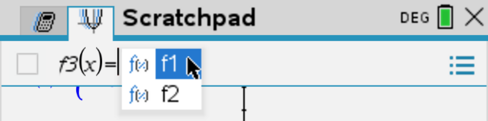
f1 using var. Supply x as the input.
x.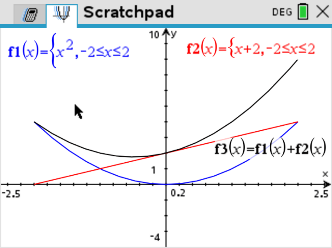
f3 label.Identify the new curve.
In this screenshot, the black curve is \(f_3\), the sum:
So \(f_3=s\).
The original parabola and line are still visible. Read the function label as well as the colour.
7.3 Hide the originals and form the difference
Worked example 6 — continued. Part B. Keep the same \(f_1\), \(f_2\) and domain; the sum is stored as \(f_3\).
Solution — Task 3
Hide the original curves without deleting their definitions.
To access an existing function entry, double-click its curve in the software, or press Tab and use the up/down arrows to move through the entries. Then select the checkbox beside the entry to show or hide that graph.

f2 is shown.
f2 is hidden.Hide f1 in the same way. Its definition is still available through var, as is the definition of f2.
Define the difference as \(f_4(x)=f_1(x)-f_2(x)\).
Open the next function-entry line. Use var to insert each stored function, enter x in each set of parentheses, and put a minus sign between the two function calls:
Press Enter. Leave f3 and f4 visible.

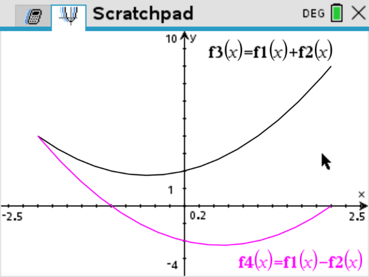
Which curve is which?
\(f_3\): the sum. Black in this screenshot:
\(f_4\): the difference. Magenta in this screenshot:
Use the displayed labels to identify the curves, including when printing in greyscale.
7.4 Check values on the calculator page
Worked example 6 — continued. Part B. Use \(f_3=s\) for the sum and \(f_4=d\) for the difference.
Solution — Task 4
Evaluate the stored functions at \(x=1\).
Use Scratchpad Calculate for a clear numerical check. There is no need to move a trace cursor along either curve.
- Select the calculator icon at the top left of Scratchpad, staying in the same Scratchpad so the stored functions remain available.
- Press var, select
f3, and insert it. - Type
1inside the parentheses to obtainf3(1), then press Enter. The result is \(4\). - Press var again, insert
f4, and evaluatef4(1). The result is \(-2\).
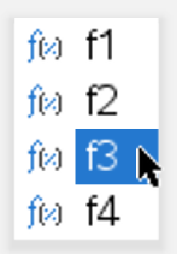
f3; repeat with f4.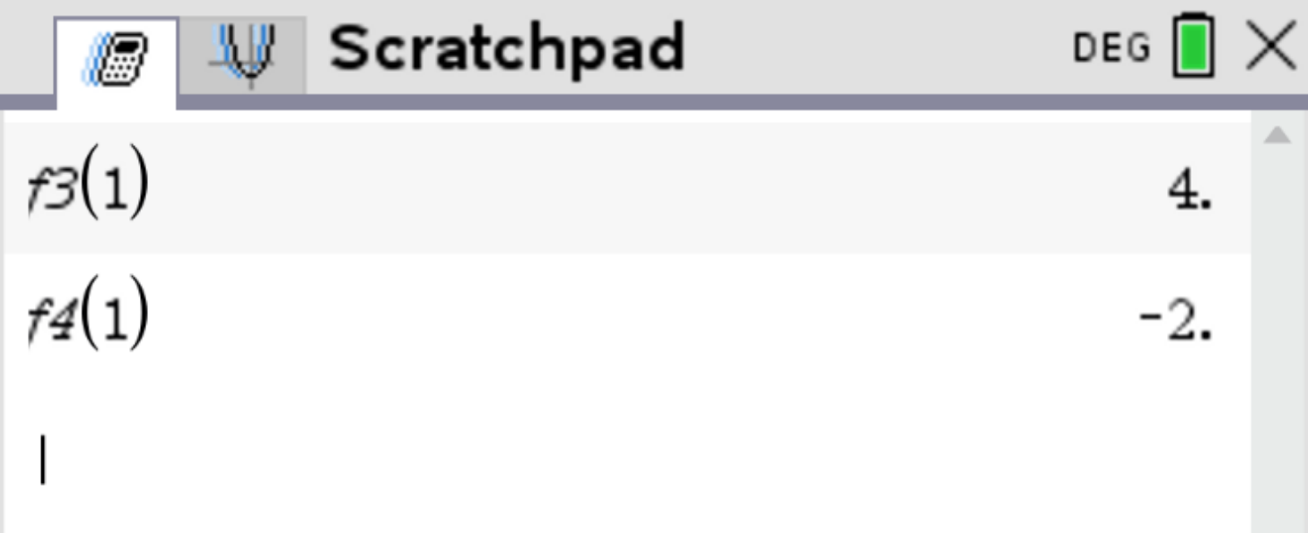
Check against the algebra. We already know that \(f(1)=1\) and \(g(1)=3\), so
The negative difference means \(f(1)\) is \(2\) less than \(g(1)\). It is not an error or a negative distance.
7.5 Finish with clear paper sketches
Worked example 6 Part B, Task 5: finished sketches
Sketch \(s(x)=x^2+x+2\) and \(d(x)=x^2-x-2\), each on \([-2,2]\). Label endpoints, intercepts, minimum points and the checked points at \(x=1\).
Supplied features: \(s\) has minimum \(\left(-\tfrac12,\tfrac74\right)\) and no x-intercepts; \(d\) has minimum \(\left(\tfrac12,-\tfrac94\right)\) and zeros at \(x=-1\) and \(x=2\).
Solution — Task 5
Sketch the same sum and difference. Use the table in 6.2 for the endpoints and y-intercepts, and the checks in 7.4 for the points at \(x=1\). Use the supplied features for the remaining labels; finding them with analysis tools is treated in IB syllabus section 2.4.
Sum: \(y=s(x)\), stored as \(f_3\)
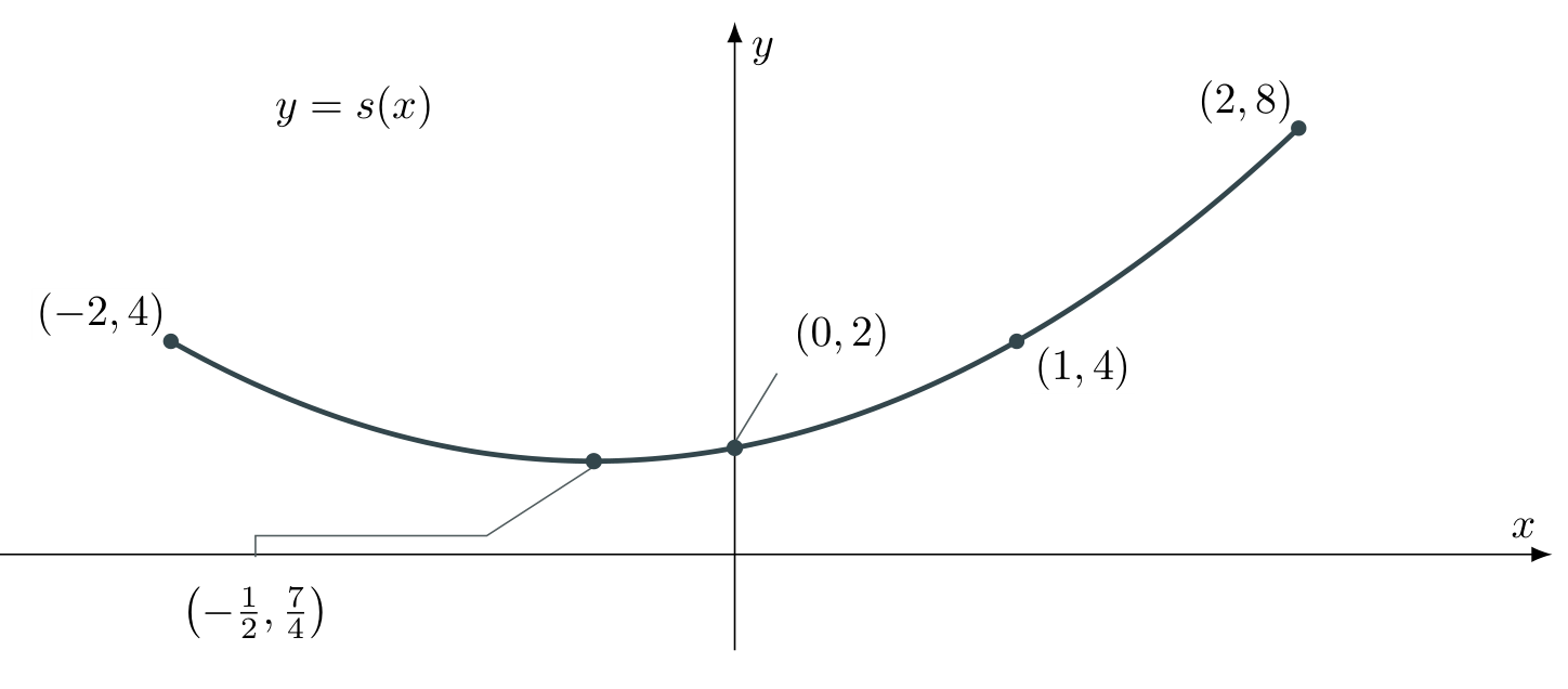
The entire sum graph lies above the x-axis: its lowest output is \(\tfrac74>0\).
Difference: \(y=d(x)\), stored as \(f_4\)
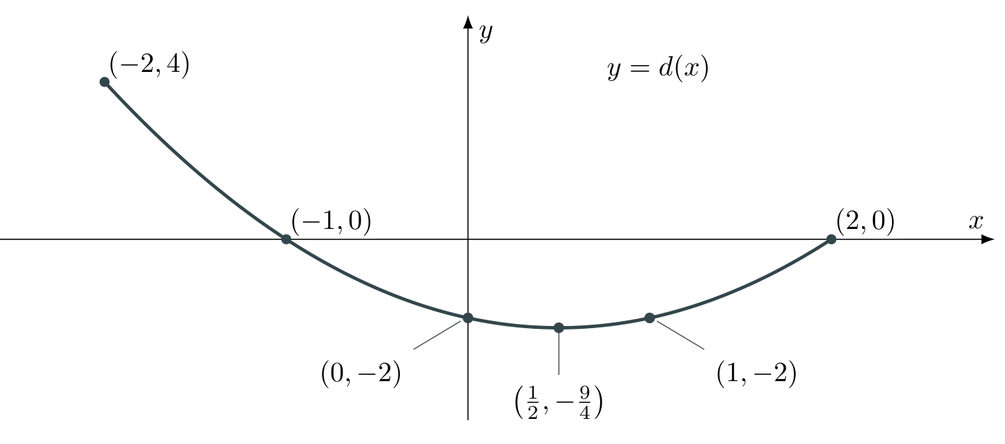
Practice
8.1 Core practice: Questions 1–6
Work on separate paper. GDC marks questions that require graphing technology; other questions can be completed without it. Label axes, relevant points and units in every sketch.
1 Points on a graph
Let \(f(x)=2x^3+1\) on \([-1,1]\).
- Find \(f(-1)\), \(f(0)\) and \(f(1)\), and state the corresponding coordinates.
- Sketch \(y=f(x)\), labelling these three points and the endpoints.
- Explain why \((1,2)\) is not on the graph.
2 Use the information given
A smooth, continuous function \(h\) has domain \([-3,3]\). Its endpoints are \((-3,2)\), \((3,-2)\); it has a local minimum at \((-1,-2)\), a local maximum at \((1,2)\), and intercepts \((-2,0)\), \((0,0)\), \((2,0)\). It decreases on \((-3,-1)\), increases on \((-1,1)\), then decreases on \((1,3)\).
- Sketch a possible graph.
- Should you add continuation arrows at the endpoints? Explain.
3 A journey
A student walks away from home at a constant speed, reaching a distance of 600 metres after 5 minutes. She waits there for 3 minutes, then returns home at a constant speed over the next 4 minutes.
- Sketch distance from home \(d\) against time \(t\), including units.
- Explain why the final segment slopes down even though she is walking.
4 A misleading window GDC
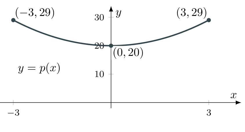
Graph \(p(x)=x^2+20\) on \([-3,3]\).
- Explain why the window \(-10\leq x\leq10\), \(-10\leq y\leq10\) appears blank.
- Choose a suitable window and sketch the required graph. Label the endpoints and the lowest point, whose input is \(x=0\).
5 Sums, differences and the shared domain GDC
Let \(f(x)=x^2+1\) on \([-2,3]\), and \(g(x)=2x\) on \([0,4]\).
- State the domain of \(s=f+g\) and \(d=f-g\).
- Find \(s(x)\), \(d(x)\), \(s(2)\) and \(d(2)\).
- Graph \(s\) and \(d\) on their common domain. Sketch them separately, labelling endpoints and the points at \(x=1,2\).
6 An unfamiliar function GDC
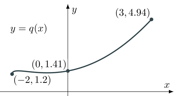
Let \(q(x)=\sqrt{x+2}+0.3x^2\), for \(-2\leq x\leq3\).
- Graph the function and find \(q(-2)\), \(q(0)\) and \(q(3)\).
- Sketch the graph, labelling these points. Inspect near the left endpoint: does the graph increase throughout the domain?
8.2 Independent checks: Questions 7–9
Complete these without following a worked solution. Use graph paper for Question 7; the graph and information supplied in Question 8 are sufficient, so no calculator is needed.
7 Draw accurately, then explain the difference
The function \(p(x)=x^2-2x\) is defined on \([-1,3]\). Its minimum point is \((1,-1)\).
| \(x\) | \(-1\) | \(0\) | \(1\) | \(2\) | \(3\) |
|---|---|---|---|---|---|
| \(p(x)\) | \(3\) | \(0\) | \(-1\) | \(0\) | \(3\) |
- Draw the graph accurately, using 2 cm for 1 unit on the x-axis and 1 cm for 1 unit on the y-axis. Label the axes, endpoints, intercepts and minimum point.
- State what could change, and what must stay correct, if the command were sketch instead.
8 From a graphing window to a restricted sketch
The display below shows part of \(y=g(x)\). A new function \(h\) has the same outputs as \(g\), but only for \(-1\leq x<3\):
You do not need to find an equation for \(g\). Use the displayed curve and its supplied features.
- On separate axes, sketch only the part of this curve for \(-1\leq x<3\) and label it \(y=h(x)\). Label the axes, both endpoint coordinates, the y-intercept and the maximum point. Use open or filled circles to show whether each endpoint is included.
- State the x-intercept of \(h\). Explain why \(h\) has only one x-intercept although \(g\) has two.
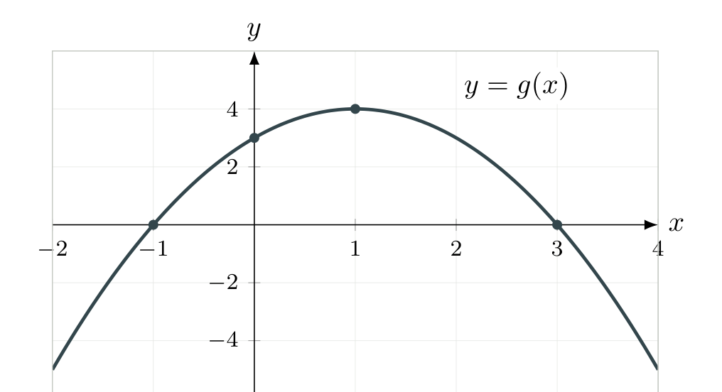
Supplied features of \(g\)
x-intercepts: \((-1,0)\) and \((3,0)\).
y-intercept: \((0,3)\).
Maximum point: \((1,4)\).
The window shows inputs from \(-2\) to \(4\). This is a viewing window, not the domain of \(h\). Use the interval stated in the question.
9 Find and correct the sketching errors
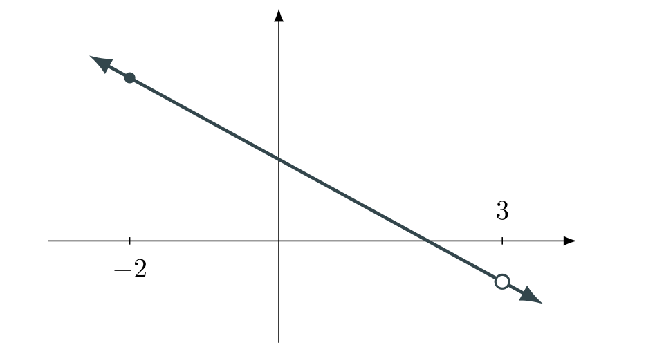
A student is asked to sketch \(k(x)=2-x\), for \(-2<x\leq3\), and produces the diagram below.
- Identify at least four errors or omissions in the student’s sketch.
- Draw a corrected sketch, labelling the axes, endpoint coordinates and intercepts.
Answers and guidance
Open each answer after attempting the question. The “Check answer” buttons in Section 8 show the same full solution without moving you away from the question.
9.1 Core practice: Questions 1–3
Question 1 — Points on a graph
1(a) Substitute into \(f(x)=2x^3+1\):
The points are \((-1,-1)\), \((0,1)\) and \((1,3)\).
1(b) The graph is a smooth increasing cubic segment, with included endpoints.
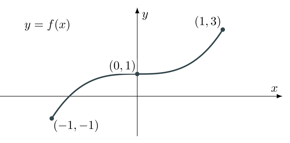
1(c) At input \(1\), the function gives output \(3\), not \(2\). Thus \((1,2)\) does not satisfy \(y=f(x)\).
Question 2 — Use the information given
2(a) One possible sketch is shown below. The order of the intercepts and turns must agree with the question.
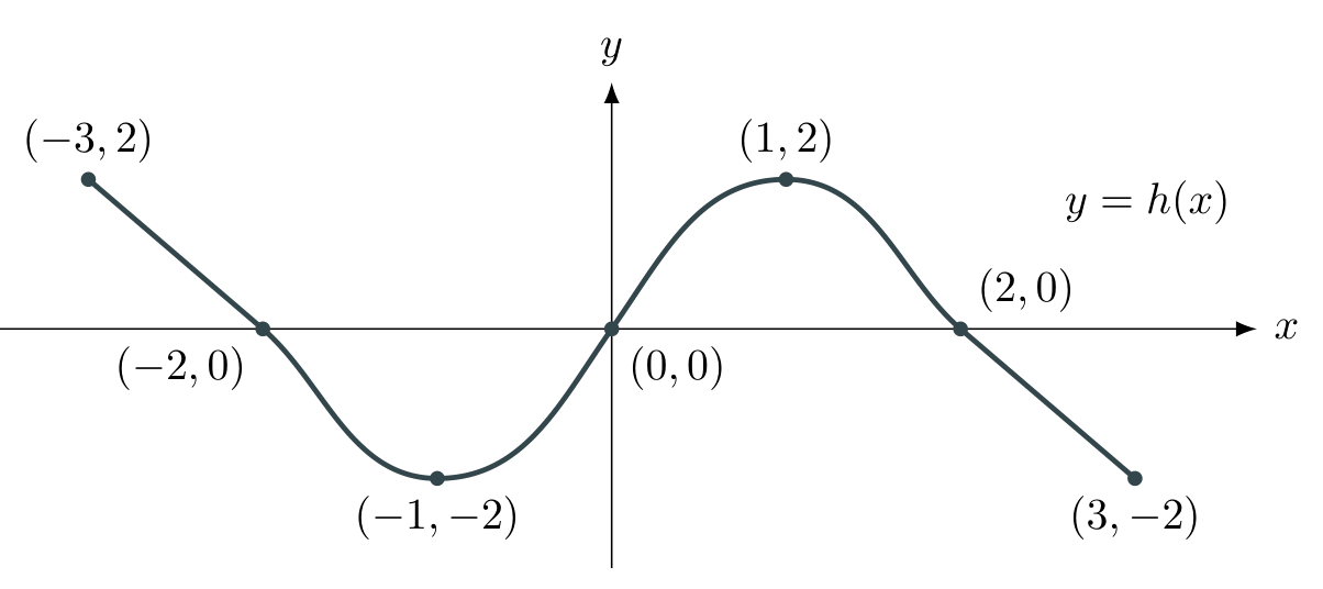
2(b) No. The stated domain ends at \(-3\) and \(3\); use filled endpoints because both are included.
Question 3 — A journey
3(a) Join \((0,0)\), \((5,600)\), \((8,600)\) and \((12,0)\) with straight segments. The waiting period ends at \(5+3=8\) minutes.
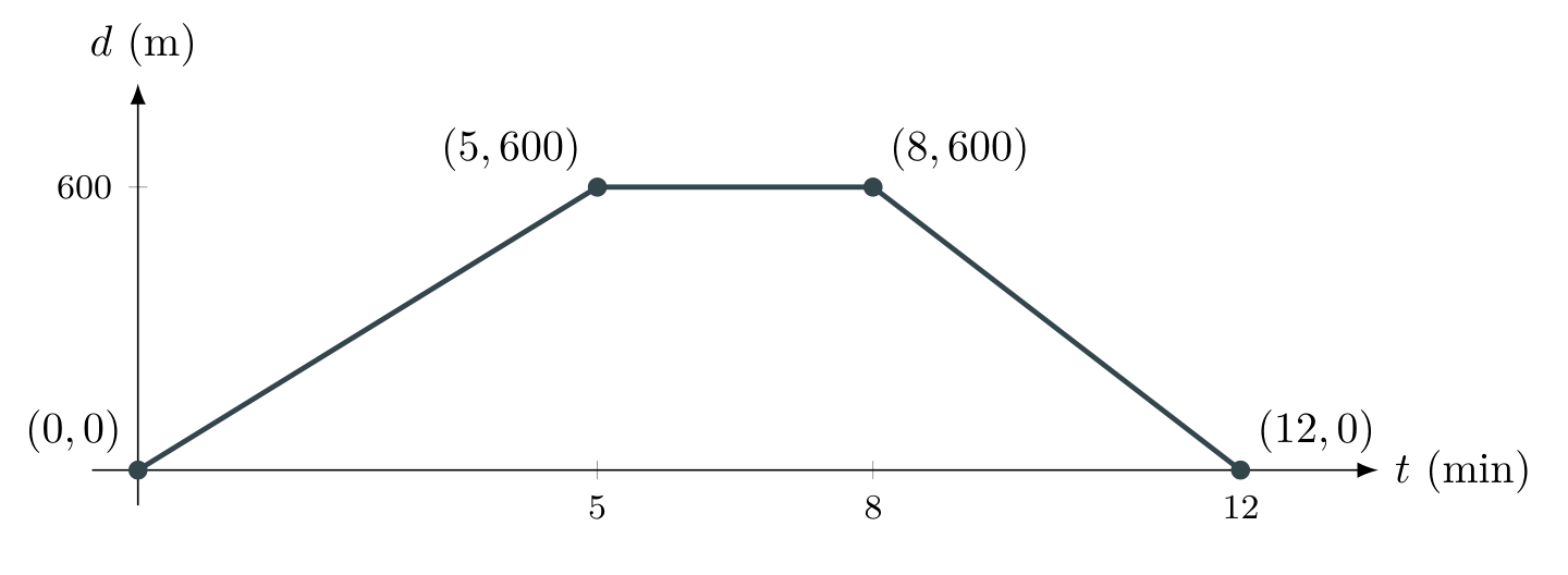
3(b) The vertical axis measures distance from home, which decreases as she returns. It does not measure the total distance she has walked.
9.2 Core practice: Questions 4–6
Question 4 — A misleading window
4(a) Since \(x^2\geq0\), every output satisfies \(p(x)\geq20\). The first window shows only \(-10\leq y\leq10\), so the curve lies above the screen.
4(b) One useful window is \(-4\leq x\leq4\), \(-2\leq y\leq32\). On the required domain, the endpoints are \((-3,29)\), \((3,29)\), and the lowest point is \((0,20)\).
Question 5 — Sums, differences and the shared domain
5(a) The domains overlap on \(\boxed{[0,3]}\).
5(b)
Thus \(s(2)=9\) and \(d(2)=1\).
5(c) Use filled endpoints and retain the common domain even after simplifying.
Question 6 — An unfamiliar function
6(a)
The approximate values are given to 3 significant figures.
6(b) No. A closer view reveals a small rise near \(x=-2\), then a fall, followed by a rise. A coarse window can hide this behaviour.
For the whole graph, one useful window is \(-2.5\leq x\leq3.5\), \(0\leq y\leq6\). Inspect the small changes with \(-2\leq x\leq0\), \(1\leq y\leq1.6\).
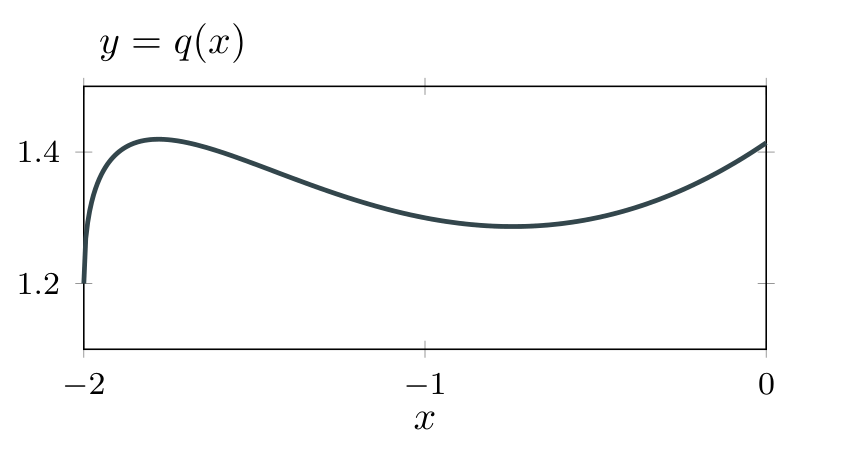
For example, \(q(-1.8)\approx1.419\) but \(q(-1)=1.300\). Increasing the input can decrease the output, so the function is not increasing throughout.
9.3 Independent checks: Questions 7 and 8
Question 7 — Accurate drawing and sketching
7(a) Accurate drawing. Plot the five supplied points and join them with a smooth parabola. The domain \([-1,3]\) includes both endpoints, so use filled circles and stop there.
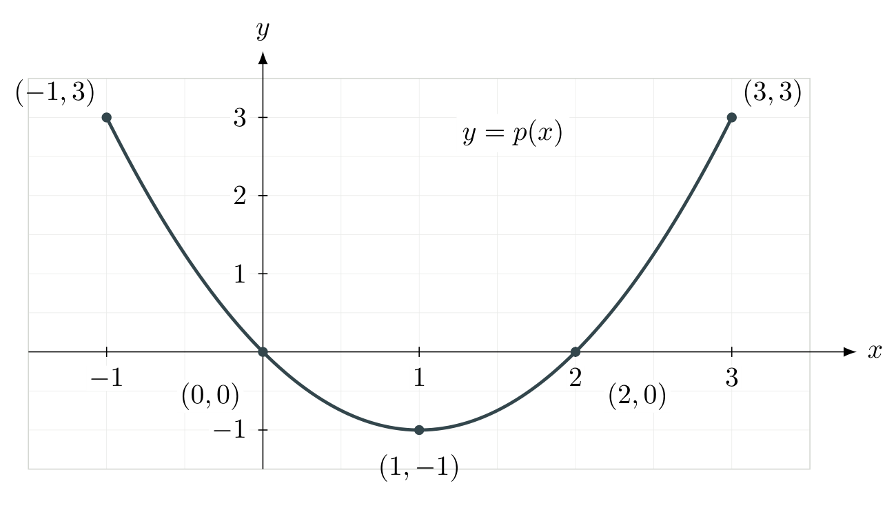
Scale on this webpage: the diagram resizes to fit your screen. For your accurate drawing, use graph paper with 2 cm per horizontal unit and 1 cm per vertical unit; do not measure the on-screen image. The printed handout uses these centimetre scales at 100% / actual-size printing.
7(b) A sketch need not use the specified centimetre scale or a grid. It must still preserve the smooth U-shape, the positions and order of the features, the labelled coordinates and the domain. “Sketch” does not mean a mathematically careless drawing.
Question 8 — Restricting the displayed graph
8(a) Keep the same curve, but only for \(-1\leq x<3\). Every retained point has the same height as on \(y=g(x)\). Omit the portions with \(x<-1\) and \(x\geq3\), and label the remaining graph \(y=h(x)\).
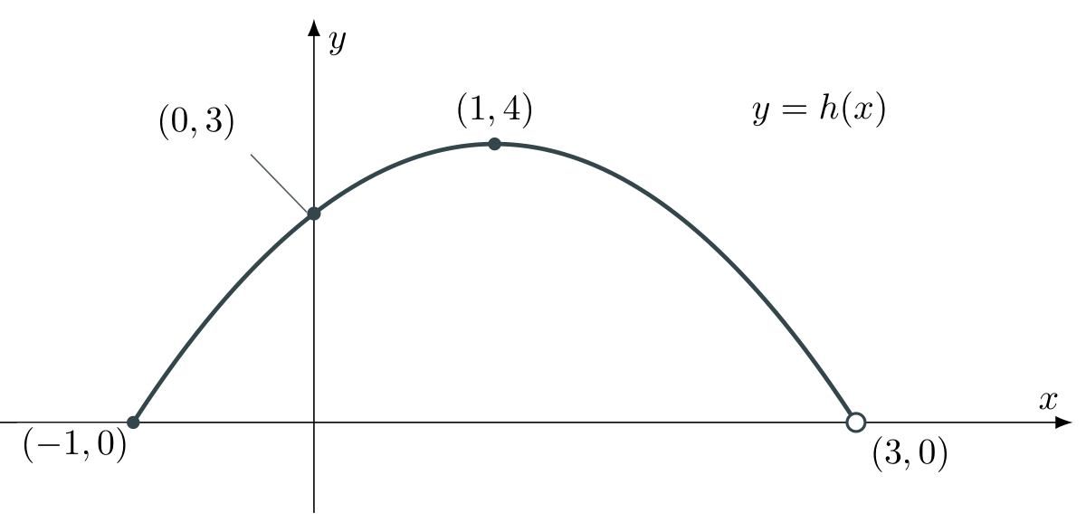
Use a filled circle at \((-1,0)\) because \(-1\) is included, and an open circle at \((3,0)\) because \(3\) is excluded. The y-intercept is \((0,3)\), and the maximum point remains \((1,4)\). There are no continuation arrows on the curve.
8(b) The only x-intercept of \(h\) is \(\boxed{(-1,0)}\). Although \(g(3)=0\), the domain of \(h\) excludes \(x=3\). The open circle at \((3,0)\) marks an excluded endpoint; it is not a point on the graph of \(h\) and is not an intercept.
9.4 Question 9 and your final self-check
Question 9 — Correcting the sketch
9(a) Errors and omissions. Four distinct issues are:
- The endpoint at \(x=-2\) is filled, but \(-2\) is excluded: it must be open.
- The endpoint at \(x=3\) is open, but \(3\) is included: it must be filled.
- The line extends beyond its allowed domain in both directions. Remove those extensions and the continuation arrows on the line.
- The axes and important coordinates are not labelled. Add \(x\), \(y\), the endpoint coordinates and both intercepts.
The arrows on the axes are appropriate and should remain.
9(b) Corrected sketch. Find the endpoint coordinates using the function’s equation:
The position \((-2,4)\) is marked with an open circle; the excluded input means \(k(-2)\) is not defined. The intercepts are \((0,2)\) and \((2,0)\).
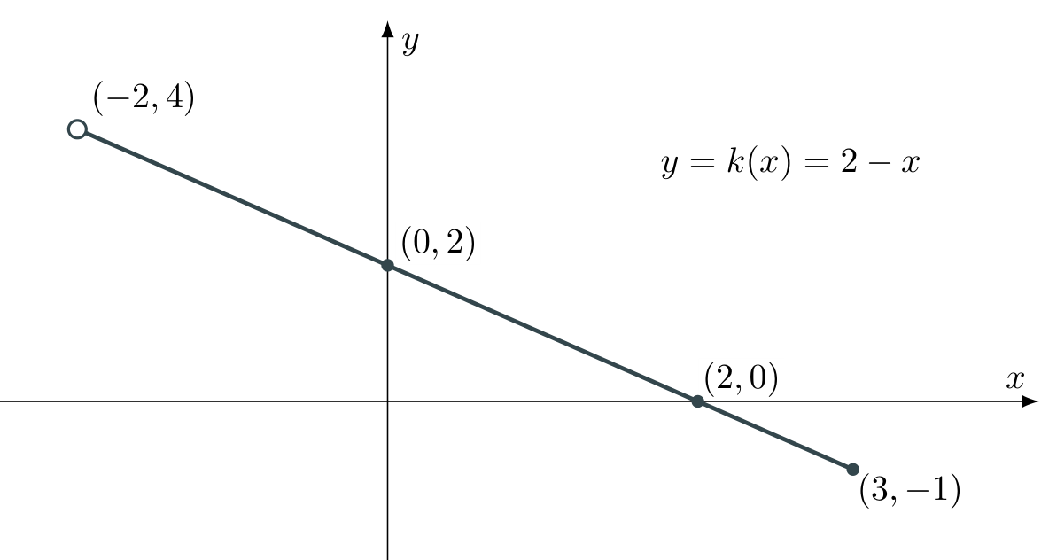
If one item is not yet secure, revisit its example and retry the matching practice question before looking at the answer. IB syllabus section 2.4 develops the calculator methods for locating key features.
Content adapted from the approved Radford Mathematics Section 2.3 handout. Syllabus references: AA guide, printed page 38; AI guide, printed page 36. Calculator screenshots and mathematical diagrams: Radford Mathematics.