IB Mathematics · Analysis and Approaches · Standard Level · Topic 4
Measures of centre and spread
Calculate a typical value, measure consistency and explain what the statistics tell you about a data set.
Learning goal
Choose a measure of centre and a measure of spread, calculate each one and explain what each tells you about the data.
Syllabus link
AA SL · SL 4.3. Measures of central tendency and dispersion, grouped estimates and changes to every observation.
Big idea
Two sets of measurements can have the same average and give very different levels of consistency.
Study route
Centre and frequency tables, spread, TI-Nspire CX, changing every value, then independent practice with worked answers.
What can an average hide?
Two dispensers are set to deliver 50 grams of coffee. Which one fills more consistently?
Each dot represents one fill. Both plots use the same horizontal scale.
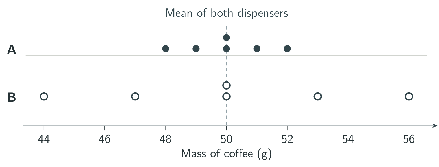
The six fills from A total \(300\) g, as do the six from B. Both means are therefore \(300/6=50\) g. A stays within \(2\) g of the target while B ranges as far as \(6\) g from it. A is the more consistent dispenser.
Mean, median and mode
Which number best describes a typical observation? It depends on the question.
Mean \(\bar{x}\)
The mean is the sum of all the values divided by the number of values there are.
Here \(n\) is the number of observations. The symbol \(\sum\) means add them all together, so the numerator is the total of the values.
Quick example · Mean
Find the mean of \(2,4,4,6\).
Solution
Add all four values, counting the value \(4\) twice, and divide by four.
Median
First write the data in increasing order, from smallest to biggest. Count every observation, including repeated values. If there are \(n\) observations, the position of the median is
In words, add one to the number of observations, then divide by two. Use the resulting position to locate the median in your increasing list.
- If \(p\) is a whole number, take the value in that position.
- If \(p\) ends in \(0.5\), take the mean of the values in the two positions on either side.
Quick example · Odd number of values
Find the median of \(8,2,6,3,9\).
Solution
First write the five values in increasing order, from smallest to biggest.
The third value is \(6\), so the median is \(6\).
Quick example · Even number of values
Find the median of \(2,3,3,7,7,9\), already in increasing order from smallest to biggest.
Solution
There are six values, giving
Position \(3.5\) is halfway between the 3rd and 4th positions. Those values are \(3\) and \(7\), so
A median can lie between two values in the list.
Mode
The mode is the value or category that occurs most often. More than one value can tie for the mode. If every value occurs just once, we usually report no mode.
Quick example · Mode
Find the modes of \(2,4,4,6\) and of \(2,3,3,7,7,9\).
Solution
The value \(4\) occurs twice, so the first list has mode \(4\).
Both \(3\) and \(7\) occur twice in the second list, so both are modes.
Worked example 1 · How long does a passenger typically wait?
A passenger records seven waiting times, in minutes, of \(6,4,12,3,8,4,5\).
- Find the mean, median and mode.
- One waiting time was recorded incorrectly. Replace the \(12\)-minute wait by a \(33\)-minute wait. Find the three corrected measures.
- Which measure would you use to describe an ordinary wait that week? Justify your answer.
Worked solution
Solution
-
In increasing order, from smallest to biggest, the times are
\[3,\;4,\;4,\;\boxed{5},\;6,\;8,\;12.\]The seven values add to \(42\), giving
\[\bar{x}=\frac{42}{7}=6\ \mathrm{min}.\]The median position is
\[p=\frac{7+1}{2}=4.\]The fourth value gives a median of \(5\) min. The mode is \(4\) min because \(4\) occurs twice.
-
Replace the recorded \(12\)-minute wait with \(33\) minutes. This adds the extra waiting time for that journey to the week's total.
\[33-12=21\ \mathrm{minutes}.\]The total minutes waited during the week increase by \(21\). The original total was \(42\) minutes. Add \(21\) minutes and divide by the same seven waiting times.
\[\bar{x}=\frac{42+21}{7}=\frac{63}{7}=9\ \mathrm{min}.\]There are still seven values, so the median is still in position \(4\). Its value is still \(5\) min, and the mode is still \(4\) min.
The median of \(5\) min is a sensible description of an ordinary wait. The unusually long wait pulls the mean upwards. For the total waiting time, the mean gives \(7\times9=63\) minutes.
Exact statistics from a frequency table
A frequency tells us how many times a value contributes to the data.
Adding all the frequencies gives the total number of observations.
Here \(n\) is the total number of values there are, counting repetitions. With indexed notation, the same sum is written \(\sum f_i\).
Multiply each value \(x_i\) by its frequency \(f_i\). Add these contributions to find the total of all observations, then divide by the sum of the frequencies.
The numerator adds all the values, allowing for repetitions. The denominator counts how many observations there are.
The IB formula booklet writes this denominator as \(n\), the total frequency.
A cumulative frequency is a running total. It locates observations in the list written in increasing order, from smallest to biggest.
Tutorial · TI-Nspire CX
TI Nspire CX – Frequency Tables, Mean, Median, Mode, Lower & Upper Quartile, IQR, Box Plot
Use frequencies to calculate the summary statistics and IQR.
Worked example 2 · Books borrowed in one month
Twenty students record how many library books they borrowed in October.
| Books \(x_i\) | 0 | 1 | 2 | 3 | 4 |
|---|---|---|---|---|---|
| Students \(f_i\) | 2 | 8 | 5 | 4 | 1 |
- Find the mean number of books borrowed.
- Find the median and the mode. Explain how you located the median.
Worked solution
Solution
-
Multiply each number of books by the number of students who reported it.
Contributions, cumulative frequencies and positions Books \(x_i\) 0 1 2 3 4 Total Students \(f_i\) 2 8 5 4 1 20 Books contributed \(f_i x_i\) 0 8 10 12 4 34 Cumulative frequency 2 10 15 19 20 — Positions in increasing order 1–2 3–10 11–15 16–19 20 — The students borrowed \(34\) books in total. Divide by the number of students.
\[\bar{x}=\frac{34}{20}=1.7.\]The mean is \(1.7\) books per student.
-
For twenty observations, the median position is
\[p=\frac{20+1}{2}=10.5.\]Each position is a place in the full list written in increasing order, from smallest to biggest. Repeated values each occupy their own place. The table's “3–10” means that the value \(1\) appears in each of positions \(3\) through \(10\).
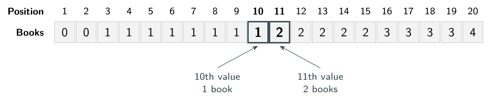
The first two groups contain \(2+8=10\) observations. Position \(10\) holds the last \(1\), and position \(11\) holds the first \(2\). Average these two book counts. The median, in books, is
\[\mathrm{median}=\frac{1+2}{2}=1.5.\]The greatest frequency is \(8\), giving a mode of \(1\) book.
Estimating a mean from grouped data
When we know only an interval, what value can we use for the observations inside it?
Represent each class by its midpoint, found by averaging its two boundaries.
Here \(L_i\) is the lower boundary and \(U_i\) is the upper boundary. Add these two boundaries and divide by two.
Quick example · Midpoint
Find the midpoint of \(10\le t<20\), with \(t\) in minutes.
Solution
The value \(15\) is halfway between the boundaries \(10\) and \(20\).
Multiply each midpoint by its frequency, add the products and divide by the total frequency.
Worked example 3 · Training sessions recorded in intervals
A coach records the durations of \(20\) individual swimming sessions.
| Duration \(t\) (min) | \(0\le t<10\) | \(10\le t<20\) | \(20\le t<30\) | \(30\le t<40\) |
|---|---|---|---|---|
| Frequency | 3 | 8 | 6 | 3 |
- State the modal class.
- Estimate the mean duration of a session.
- Explain why the exact mean cannot be recovered from this table.
Worked solution
Solution
The classes have equal width. The greatest frequency is \(8\), so the modal class is \(10\le t<20\) minutes. Report the whole interval. The individual durations within it are unknown.
-
Calculate the midpoint of each interval and weight it by its frequency.
Midpoint calculation Midpoint \(m_i\) (min) 5 15 25 35 Total Frequency \(f_i\) 3 8 6 3 20 Estimated minutes \(f_i m_i\) 15 120 150 105 390 The estimated total is \(390\) minutes, shared across twenty sessions.
\[\bar{t}\approx\frac{390}{20}=19.5.\]The estimated mean duration is \(19.5\) minutes per session.
Calculator check. Use \(5,15,25,35\) as the values and \(3,8,6,3\) as their frequencies.
The actual times within each interval are unknown. An \(11\)-minute swim and a \(19\)-minute swim belong to the same class but contribute different amounts to the true total. Using class midpoints gives an estimate of the mean.
Quartiles and the interquartile range
How wide is the part of the distribution occupied by its middle half?
In a list written in increasing order, from smallest to biggest, the lower quartile \(Q_1\), median \(Q_2\) and upper quartile \(Q_3\) mark roughly the \(25\%\), \(50\%\) and \(75\%\) positions. With repeated values or a small data set, these percentages describe positions approximately.
To find the interquartile range, subtract the lower quartile from the upper quartile.
The IB formula booklet gives this formula under section 4.2.
Worked example 4 · The middle half of the book counts
Use technology to find \(Q_1\), \(Q_2\), \(Q_3\) and the IQR for the \(20\) students in worked example 2. Interpret the IQR in context.
Worked solution
Solution
Enter the book counts and their frequencies in One-Variable Statistics. The full calculator steps are in section 7. The output gives
For a hand-check, split the increasing list into two halves of ten. The median position within each half is
The lower half's 5th and 6th values both equal \(1\). The upper half's 5th and 6th values are \(2\) and \(3\), at full-list positions \(15\) and \(16\). Their mean is \(2.5\).
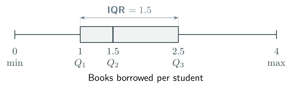
The middle half of the book counts in increasing order spans \(2.5-1=1.5\) books. The full range is \(4-0=4\) books. A quartile can lie between two observed counts.
Standard deviation and variance
How far from the mean do observations tend to lie?
A deviation measures how far a value is above or below the mean. The deviations sum to zero because positive and negative differences cancel. Squaring each difference first gives a way to measure spread.
The population variance is
In words, subtract the mean from each value, square each difference, add the squares and divide by the number of values.
The population standard deviation is
Take the square root of the variance to obtain the standard deviation, in the original units.
Use technology to find these measures in section 4.3. The calculation below explains the calculator's results. An SD of zero means all observations are the same.
Worked example 5 · Putting a number on consistency
The coffee fills from section 1, in grams, were
Dispenser A \(48,49,50,50,51,52\).
Dispenser B \(44,47,50,50,53,56\).
- Find the variance and standard deviation for dispenser A.
- Compare the dispensers using their means and standard deviations.
Worked solution
Solution
-
The mean is \(50\) g. Each squared deviation counts once.
Dispenser A's deviations from its mean of 50 g Deviation (g) \(-2\) \(-1\) 0 0 1 2 Squared deviation (\(\mathrm{g}^2\)) 4 1 0 0 1 4 The squared deviations add to \(10\). Divide by six, then take the square root.
\[\sigma_A^2=\frac{10}{6}=\frac{5}{3}\ \mathrm{g}^2.\]\[\sigma_A=\sqrt{\frac{5}{3}}\approx1.29\ \mathrm{g}.\]The calculator's \(\sigma_x\) gives the SD directly.
One-variable statistics for B gives \(\bar{x}_B=50\) g and \(\sigma_B\approx3.87\) g. Both dispensers average the target fill, but B's fills have three times A's standard deviation. A delivers a more consistent mass.
TI-Nspire CX one-variable statistics
Use the data below to calculate the summary statistics. Keep the same document open throughout this walkthrough.
Twenty students recorded how many library books they borrowed in October. The data are repeated below.
| Books borrowed \(x_i\) | 0 | 1 | 2 | 3 | 4 |
|---|---|---|---|---|---|
| Number of students \(f_i\) | 2 | 8 | 5 | 4 | 1 |
1 · Enter the data
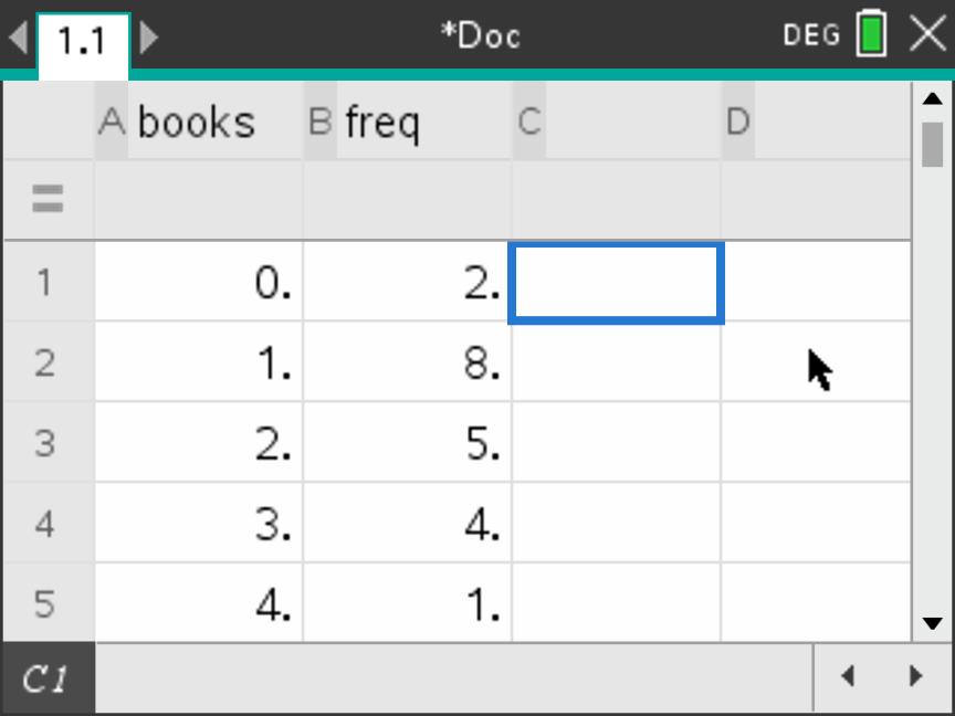
Press Home → New Document → Add Lists & Spreadsheet. Move to the name box beside A, type books and press Enter. Name column B freq in the same way. The row marked \(=\) is the formula row.
Enter the book counts starting at A1 and the frequencies starting at B1. Press Enter after each value. Include \(0\) in A1 because two students borrowed zero books.
2 · Open One-Variable Statistics
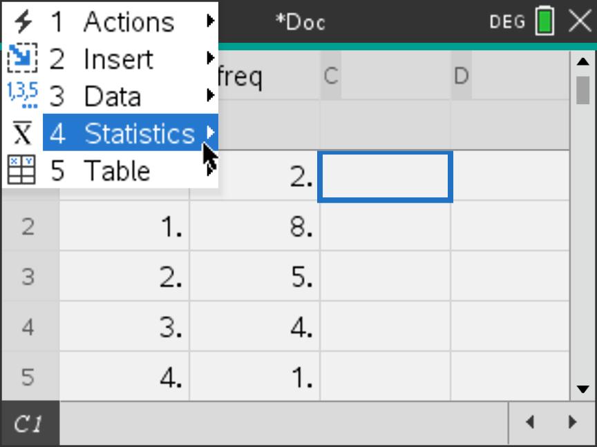
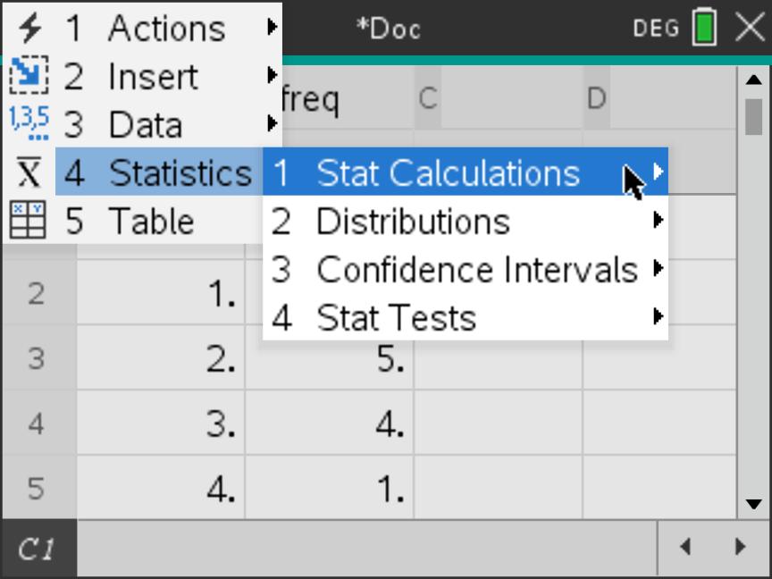
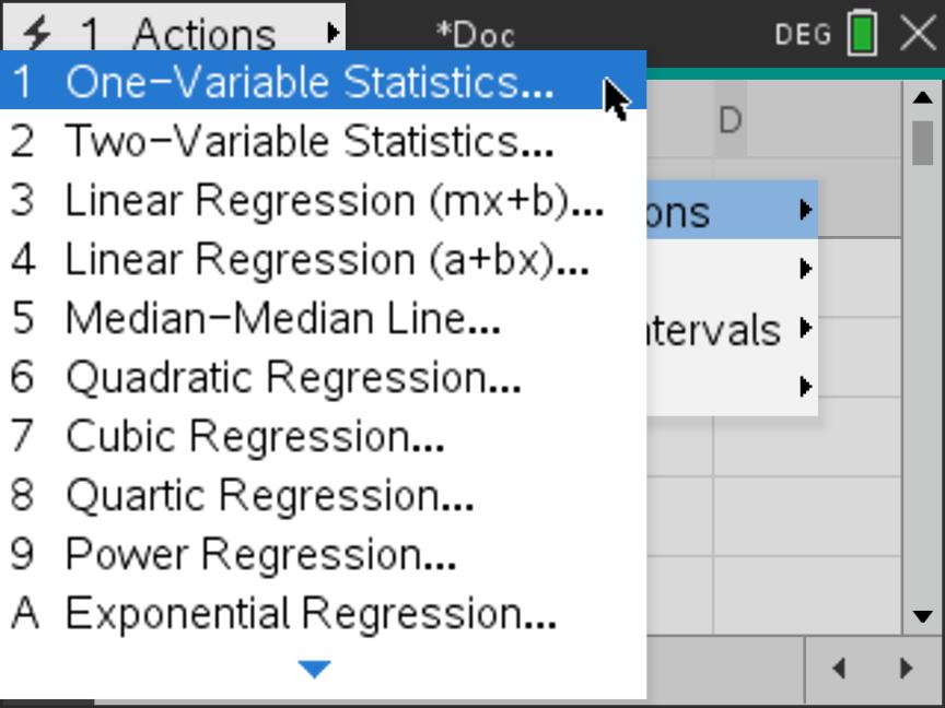
From the spreadsheet, choose Menu → Statistics → Stat Calculations → One-Variable Statistics. The shortcut is Menu 4 1 1. The three menu choices are shown in order below.
Raw-data calculator tutorial
Enter a raw data list and read the mean, median and quartiles.
3 · Choose the lists and run the calculation
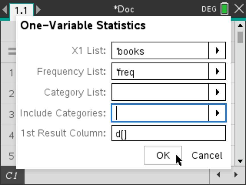
Set Num of Lists to \(1\), then select OK. The measured quantity is the number of books borrowed. The frequencies tell the calculator how many times to count each value. The next dialogue selects those two lists.
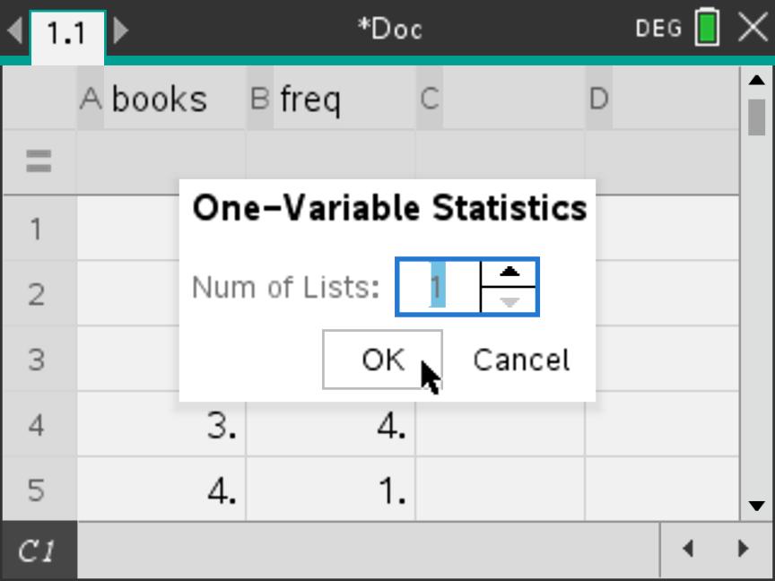
| X1 List | Select books. |
|---|---|
| Frequency List | Select freq. |
| Category fields | Leave Category List and Include Categories blank. |
| 1st Result Column | Set this to d[] as shown. Result labels appear in column D and values in column E. Select OK. |
4 · Read the mean and standard deviation
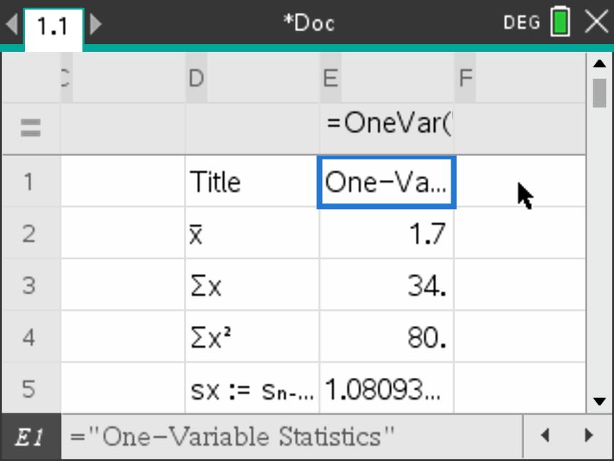
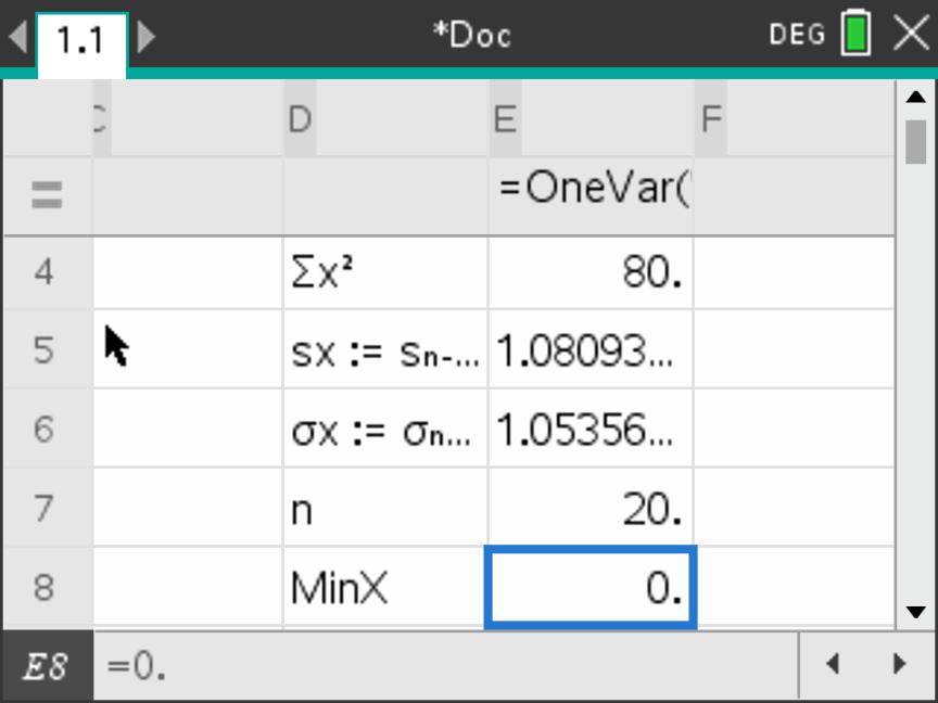
Move across to columns D and E if needed. The mean is \(1.7\) books per student. Scroll down to \(\sigma_x\), the population standard deviation, and check that \(n=20\). A reading of \(n=5\) means each book count was included just once, so check the frequency setting.
5 · Read the quartiles
Scroll further down to \(Q_1X\), \(\mathrm{Median}X\) and \(Q_3X\). These give the lower quartile, median and upper quartile. The table summarises the results for the twenty students.
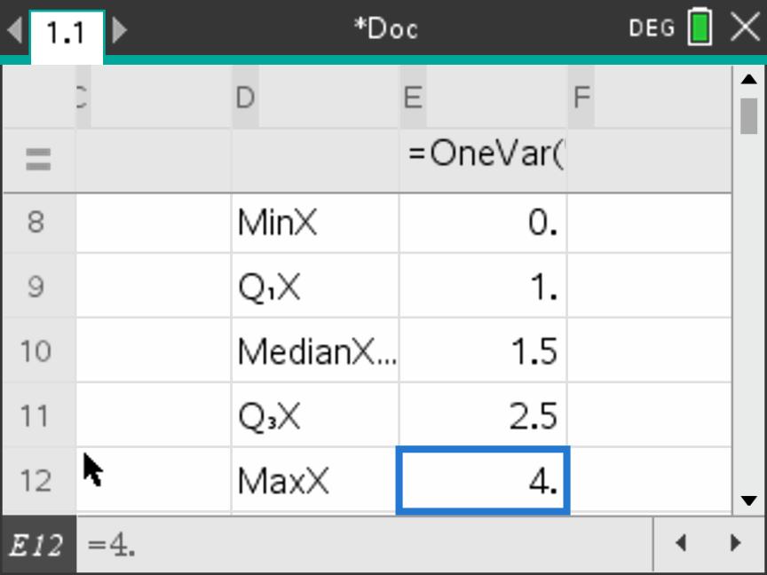
| Measure | Value |
|---|---|
| Mean \(\bar x\) | \(1.7\) |
| Population SD \(\sigma_x\) | \(1.053565\ldots\) |
| Sample SD \(s_x\) | \(1.080935\ldots\) |
| Observations \(n\) | \(20\) |
| Minimum | \(0\) |
| Lower quartile \(Q_1\) | \(1\) |
| Median \(Q_2\) | \(1.5\) |
| Upper quartile \(Q_3\) | \(2.5\) |
| Maximum | \(4\) |
6 · Calculate variance without rounding early
The dots in a result cell indicate further stored digits. Use the stored standard deviation when calculating variance.
- From spreadsheet page 1.1, press Ctrl + Doc, then choose 1 Add Calculator. The new page is 1.2. Both pages belong to problem 1 and share its stored values.
- Press var. Highlight \(\mathtt{stat.}\sigma_x\) with the arrow keys, then press Enter to paste it into the input line.
- Press the square key \(\boxed{x^2}\), then Enter.
- Check that the result is \(1.11\). Give the variance in squared units.
Expected calculation using the stored value
The variance is measured in \(\mathrm{books}^2\).
If the stored statistic is unavailable, return to the spreadsheet and run One-Variable Statistics in this problem. For the IQR, subtract the quartiles.
Changing every observation
Can you predict the new statistics without entering the entire list again?
Start with the four values \(4,4,6,6\). Their mean and median are \(5\), their IQR is \(2\), their standard deviation is \(1\) and their variance is \(1\).
Quick example · Add the same amount
Add \(3\) to each of \(4,4,6,6\). Find the new mean, standard deviation and variance.
Solution
The new values are \(7,7,9,9\). Each value moves up by \(3\), so the mean also moves up by \(3\).
Each value is still one unit from its mean. The gaps between values are preserved, so the spread stays the same.
Quick example · Multiply by the same number
Double each of the original values \(4,4,6,6\). Find the new mean, standard deviation and variance.
Solution
The new values are \(8,8,12,12\). Their mean doubles.
Each value is now two units from its mean. Distances double, so the SD doubles. Squaring the new SD gives the new variance.
| Data | Mean | IQR | SD | Variance |
|---|---|---|---|---|
| Original \(4,4,6,6\) | 5 | 2 | 1 | 1 |
| Add \(3\) to every value | 8 | 2 | 1 | 1 |
| Double every original value | 10 | 4 | 2 | 4 |
Adding or subtracting a constant moves the centre and preserves spread. Multiplying all values by a positive constant scales both the centre and the distances between values. Variance scales by the square of that constant.
General rules and application
Suppose every value \(x\) is replaced by a new value \(y\), according to
Adding \(b\) moves every point the same distance, preserving the gaps between points. Multiplication by \(a\) multiplies lengths of gaps by \(|a|\). Because variance is a squared measure, its scale factor is \(a^2\).
| Statistic | Formula for the changed data |
|---|---|
| Mean | \(\bar{y}=a\bar{x}+b\) |
| Median | \(M_y=aM_x+b\) |
| IQR | \(\mathrm{IQR}_y=|a|\mathrm{IQR}_x\) |
| Standard deviation | \(\sigma_y=|a|\sigma_x\) |
| Variance | \(\sigma_y^2=a^2\sigma_x^2\) |
For \(a\ne0\), each mode \(m\) becomes \(am+b\), because the frequency of a value is preserved. For \(a>0\), each quartile changes to \(aQ+b\). For \(a<0\), order reverses. The old upper quartile gives the new lower quartile and vice versa. If \(a=0\), all values equal \(b\) and all measures of spread are zero.
Worked example 6 · Calibrating a temperature sensor
A sensor's readings \(x\) have mean \(16\,{}^\circ\mathrm{C}\), median \(15\,{}^\circ\mathrm{C}\), IQR \(5\,{}^\circ\mathrm{C}\) and SD \(2\,{}^\circ\mathrm{C}\). The corrected reading is \(y=1.2x-3\) in degrees Celsius.
- Find the corrected mean and median.
- Find the corrected IQR, SD and variance.
Worked solution
Solution
-
Apply both operations to the measures of centre.
\[\bar{y}=1.2(16)-3=16.2\,{}^\circ\mathrm{C}.\]\[M_y=1.2(15)-3=15\,{}^\circ\mathrm{C}.\] -
Multiplying each reading by \(1.2\) increases each gap by a factor of \(1.2\). Subtracting \(3\) preserves those gaps.
\[\mathrm{IQR}_y=1.2(5)=6\,{}^\circ\mathrm{C}.\]\[\sigma_y=1.2(2)=2.4\,{}^\circ\mathrm{C}.\]Square the corrected SD to find the corrected variance.
\[\sigma_y^2=(2.4)^2=5.76\ ({}^\circ\mathrm{C})^2.\]
Independent practice and worked answers
Try the questions before opening their worked solutions. Give exact answers where convenient and otherwise round to three significant figures. Use the working to locate any discrepancy in your own calculations.
1 · A typical delivery time
Seven delivery times, in minutes, are \(14,\ 12,\ 16,\ 21,\ 12,\ 15,\ 13\).
- Calculate the mean, median and mode.
- The recorded value \(21\) should be \(49\). Find the corrected mean and median.
- Choose a measure to describe a typical delivery after the correction. Explain your choice.
Show worked solution
Solution
-
In increasing order, from smallest to biggest, the times are \(12,12,13,14,15,16,21\). Add the times and divide by seven.
\[\bar{x}=\frac{103}{7}\approx14.7\ \mathrm{min}.\]The median position is
\[p=\frac{7+1}{2}=4.\]The fourth value is \(14\), giving a median of 14 minutes. The mode is 12 minutes.
-
Replacing \(21\) by \(49\) increases the total by \(28\) minutes.
\[\bar{x}=\frac{103+28}{7}=\frac{131}{7}.\]\[\bar{x}\approx18.7\ \mathrm{min}.\]The fourth time is still \(14\), so the median is 14 minutes.
-
The median describes a typical delivery. The unusually long \(49\)-minute wait pulls the mean upwards.
2 · Bicycle inspections
For each bicycle inspected, a mechanic records the number of faults.
| Number of faults | 0 | 1 | 2 | 3 | 4 |
|---|---|---|---|---|---|
| Number of bicycles | 3 | 5 | 4 | 3 | 1 |
- Find the number of bicycles and the mean number of faults per bicycle.
- Use cumulative frequencies to find the median. State the mode.
- Enter the values and frequencies into two named calculator lists. Check \(n\), then find \(Q_1\), \(Q_3\), the IQR, population standard deviation and variance. Use the stored SD to calculate the variance.
- Interpret the IQR in the context of the bicycle inspections.
Show worked solution
Solution
-
There are \(3+5+4+3+1=16\) bicycles. Multiply each number of faults by its frequency. The contributions to the total are \(0(3)=0\), \(1(5)=5\), \(2(4)=8\), \(3(3)=9\) and \(4(1)=4\).
The mean number of faults per bicycle is
\[\bar{x}=\frac{0+5+8+9+4}{16}.\]\[\bar{x}=\frac{26}{16}=1.625.\]The mean is 1.625 faults per bicycle.
-
With sixteen bicycles, the median position is
\[p=\frac{16+1}{2}=8.5.\]The cumulative frequencies \(3,8,12,15,16\) show that positions \(8\) and \(9\), in increasing order from smallest to biggest, have \(1\) and \(2\) faults. Average those values.
\[\mathrm{median}=\frac{1+2}{2}=1.5\ \mathrm{faults}.\]The largest frequency is \(5\), so the mode is 1 fault.
-
Select the faults list under X1 List and the bicycle counts under Frequency List. Check \(n=16\). Use the population SD and square its stored value for the variance.
Bicycle-inspection summary statistics Measure Result Lower quartile \(Q_1=1\) fault Upper quartile \(Q_3=2.5\) faults Interquartile range \(\mathrm{IQR}=2.5-1=1.5\) faults Population SD \(\sigma_x=1.165922\ldots\approx1.17\) faults Population variance \(\sigma_x^2=1.359375\approx1.36\ \mathrm{faults}^2\) -
The middle half of the ordered fault counts spans \(1.5\) faults between the lower and upper quartiles. Repeated counts make quartiles approximate positional boundaries.
3 · Queueing times
A café records queueing times \(t\), in minutes, for a group of customers.
| Time | \(0\le t<5\) | \(5\le t<10\) | \(10\le t<15\) | \(15\le t<20\) |
|---|---|---|---|---|
| Frequency | 4 | 9 | 5 | 2 |
- State the modal class and estimate the mean queueing time.
- A manager claims that exactly nine customers waited \(7.5\) minutes. Does the table establish this? Explain.
Show worked solution
Solution
-
The modal class is \(5\le t<10\) minutes. Its frequency is \(9\), the largest of the four equal-width classes. The midpoints are \(2.5\), \(7.5\), \(12.5\) and \(17.5\) minutes.
Multiplying each midpoint by its frequency gives contributions of \(4(2.5)=10\), \(9(7.5)=67.5\), \(5(12.5)=62.5\) and \(2(17.5)=35\) minutes. These add to an estimated total of \(175\) minutes for \(20\) customers.
\[\bar{t}\approx\frac{175}{20}=8.75\ \mathrm{min}.\] -
All nine waited at least \(5\) but less than \(10\) minutes. The table gives no individual times, so it cannot establish how many waited exactly \(7.5\) minutes.
4 · A calculator check
The masses of eight small parcels, in kilograms, are \(8,\ 9,\ 9,\ 11,\ 12,\ 13,\ 14,\ 16\). Treat the eight parcels as the population.
- Use one-variable statistics to find \(\bar{x},\ Q_1,\ Q_2,\ Q_3\) and the IQR.
- Read off the standard deviation and use the stored value to find the variance. Include units for both.
Show worked solution
Solution
-
Use the raw masses as the X1 List with Frequency List set to \(1\). Check \(n=8\). The mean is \(11.5\) kg. The quartiles are \(Q_1=9\) kg, \(Q_2=11.5\) kg and \(Q_3=13.5\) kg.
To check the median by hand, find its position.
\[p=\frac{8+1}{2}=4.5.\]The 4th and 5th values in increasing order, from smallest to biggest, are \(11\) and \(12\), whose average is \(11.5\) kg. Subtract the lower quartile from the upper quartile.
\[\mathrm{IQR}=13.5-9=4.5\ \mathrm{kg}.\] -
The \(\sigma_x\) reading is \(2.598076\ldots\) kg, giving an SD of 2.60 kg to three significant figures. Squaring the stored reading gives a variance of \(6.75\ \mathrm{kg}^2\).
5 · Two morning buses
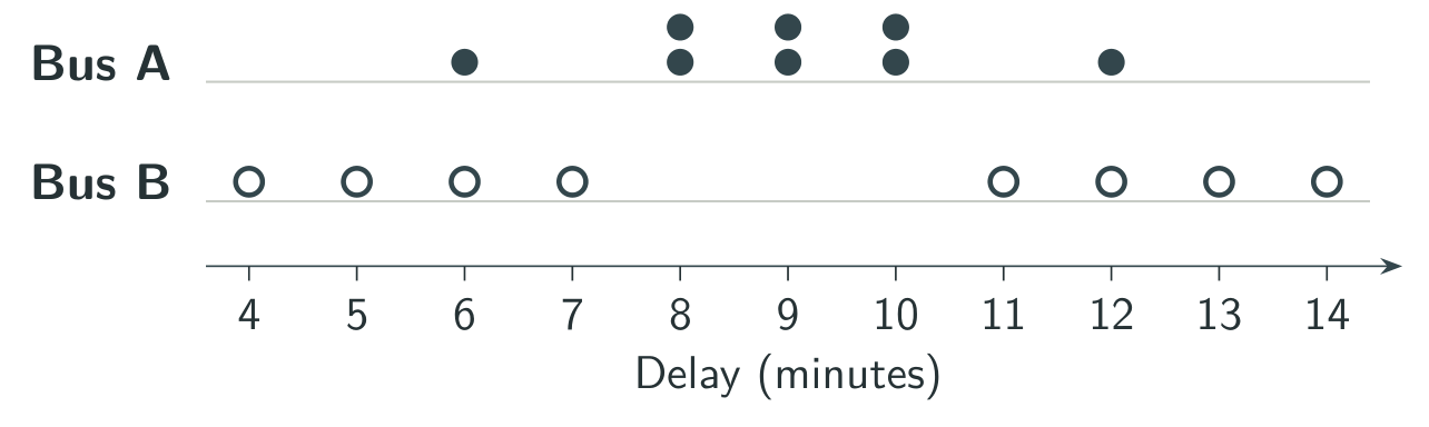
A traveller records the delay of each bus over eight mornings. Each dot is one observation.
- Find the mean and standard deviation for each bus.
- A traveller wants a predictable delay. Use both measures to justify a choice.
Show worked solution
Solution
-
The plotted delays are \(6,8,8,9,9,10,10,12\) for A and \(4,5,6,7,11,12,13,14\) for B. Each list totals \(72\) minutes. With the frequency setting at \(1\), one-variable statistics gives the following results.
Delay statistics for the two buses Measure Bus A Bus B Mean delay (min) \(72/8=9\) \(72/8=9\) Standard deviation (min) \(\sqrt{2.75}\approx1.66\) \(\sqrt{13.5}\approx3.67\) -
Choose bus A for predictability on this evidence. Its mean delay equals B’s at \(9\) minutes, and its smaller SD, \(1.66\) minutes compared with \(3.67\) minutes, means that its observed delays are more tightly clustered around the mean.
6 · A length sensor
A factory measures lengths \(x\) in centimetres. The mean is \(18\) cm, the IQR is \(0.6\) cm and the standard deviation is \(0.4\) cm. Each value is converted to millimetres, then increased by \(2\) mm to correct a calibration error.
- Write an expression for the corrected length \(y\), in millimetres, in terms of \(x\).
- Find the corrected mean, IQR, standard deviation and variance. Give the units of each.
Show worked solution
Solution
-
Convert centimetres to millimetres by multiplying by \(10\), then apply the correction.
\[y=10x+2.\] -
Apply the same operations to the mean.
\[\bar{y}=10(18)+2=182\ \mathrm{mm}.\]The \(2\) mm correction shifts every length equally, so it contributes nothing to the spread.
\[\mathrm{IQR}_y=10(0.6)=6\ \mathrm{mm}.\]\[\sigma_y=10(0.4)=4\ \mathrm{mm}.\]\[\sigma_y^2=4^2=16\ \mathrm{mm}^2.\]
7 · Recovering a missing frequency
The mean score in a game is \(1.5\) points. One frequency in the table is missing.
| Score | 0 | 1 | 2 | 3 |
|---|---|---|---|---|
| Frequency | 3 | 4 | \(k\) | 2 |
- Form an equation for \(k\), and hence find the missing frequency.
- Find the median score.
- A score of \(3\) was entered in place of a \(2\). Find the corrected mean without recomputing the entire frequency table.
Show worked solution
Solution
-
The total score is \(0(3)+1(4)+2k+3(2)=10+2k\) and the number of scores is \(9+k\). Using the given mean gives
\[\frac{10+2k}{9+k}=1.5.\]\[20+4k=27+3k.\]\[k=7.\] -
There are \(16\) scores, giving a median position of
\[p=\frac{16+1}{2}=8.5.\]Positions \(8\) and \(9\), in increasing order from smallest to biggest, are both in the group of seven \(2\)s, which occupies positions \(8\)–\(14\). Their average is \(2\), so the median is 2 points.
-
The original total is \(24\) points. The correction removes one point and keeps the number of scores fixed, giving
\[\bar{x}=\frac{23}{16}=1.4375\ \mathrm{points}.\]
8 · Comparing two café queues
The waiting times of nine customers at café A, in minutes, are \(4,\ 5,\ 6,\ 6,\ 7,\ 8,\ 9,\ 10,\ 35\).
At café B, the median waiting time is \(8\) minutes and the IQR is \(2\) minutes. These quartiles were calculated using the same TI-Nspire convention.
- Use technology to find the lower quartile, median, upper quartile and IQR for café A. Check that \(n=9\).
- Explain what café A’s IQR tells you about the middle half of its waiting times.
- Compare the typical waiting time and the spread of the middle half for the two cafés. Use the median and IQR in your answer.
- Explain why the median and IQR are informative for café A’s data, which include the \(35\)-minute wait.
Show worked solution
Solution
-
Use the nine waiting times as the X1 List, with Frequency List set to \(1\). Check \(n=9\). The TI-Nspire output gives
\[Q_1=5.5\ \mathrm{min}.\]\[Q_2=7\ \mathrm{min}.\]\[Q_3=9.5\ \mathrm{min}.\]\[\mathrm{IQR}=9.5-5.5=4\ \mathrm{min}.\]For a hand-check, the list is already in increasing order, from smallest to biggest. The median position is
\[p=\frac{9+1}{2}=5.\]The fifth value is \(7\). Excluding it leaves halves \(4,5,6,6\) and \(8,9,10,35\). In each half, the median position is
\[p=\frac{4+1}{2}=2.5.\]Averaging the second and third values in each half gives
\[Q_1=\frac{5+6}{2}=5.5.\]\[Q_3=\frac{9+10}{2}=9.5.\]Including the median in both halves would give \(6\) and \(9\), illustrating the convention difference.
-
The middle half of A’s waiting times spans \(4\) minutes between its lower and upper quartiles, \(5.5\) and \(9.5\) minutes.
-
A has the shorter typical wait, with median \(7\) minutes compared with B’s \(8\). B has more tightly clustered central waiting times, with IQR \(2\) minutes compared with A’s \(4\).
-
The \(35\)-minute wait pulls A’s mean upwards and increases its SD. The median and IQR describe its typical wait and central spread while being less sensitive to that unusually long wait.
Before checking your answers
For an estimate, identify what was approximated. For a comparison, name the groups and put the statistics back into the context of the question.
Tutorials and references
Tutorials at a glance
- Enter raw data and read the mean, median and quartiles. Mean, Median, Lower Quartile, Upper Quartile TI NSpire CX
- Use frequency tables to find summary statistics and IQR. TI Nspire CX – Frequency Tables, Mean, Median, Mode, Lower & Upper Quartile, IQR, Box Plot
References
International Baccalaureate, Mathematics analysis and approaches guide, Topic 4, pp. 53, 55.
- Texas Instruments support guide. One-variable statistics
- Texas Instruments support guide. Calculating variance
- TI-Nspire CX reference guide. Population and sample variance commands